Line picking algorithms

Line picking

Echoview offers algorithms that are used to pick lines on single beam echograms. The algorithms can be used in two situations.

1. For an Editable line using a Line pick. The algorithm settings are entered under Single beam on the Lines and Surfaces page of the EV File Properties dialog box. See Line picking and bottom detection for further information.
   - or -
2. For a Virtual line using one of the Line pick operators. The algorithm settings are entered on the operator specific page of the Line Properties dialog box. See Creating virtual lines for further information.

Echoview supports different algorithms for picking bottom lines in single beam echograms, including:

• Trained model bottom exclusion (experimental)
• Best bottom candidate
• Maximum Sv
• Delta Sv

Detecting a boundary

Echoview offers the Threshold offset line operator algorithm to detect a vegetation boundary or other boundaries in water column data. The operator may be configured to detect either a minimum or a maximum threshold value relative to a specified (base) line.

Threshold offset

The Threshold offset detection evaluates Operand 1 sample values in a ping, starting from the line specified by Operand 2. Eligible samples have sample depths that occur in the Direction of detection from Operand 2.

1. Evaluate ( Sample value (dB ) < Threshold (dB)) by testing samples in a ping from Operand 2 in the Direction of detection. When Allow detection from echogram extents is selected begin search at the extent of Operand 1.
   1. If the depth of the potential boundary sample is less than the (Depth of Operand 2 + Minimum accepted distance (m)), continue the detection.
   2. Stop the detection if the depth of the potential boundary sample is greater than the (Depth of Operand 2 + Maximum detection distance (m)).
2. The Threshold offset line depth is assigned to the depth of the sample that is greater than the Threshold and whose depth is greater than the Minimum accepted distance and is less than the Maximum detection distance from Operand 2 in the Direction of detection. If no sample satisfies all these criteria, the Threshold offset line depth is set to the depth of Operand 2.
3. Proceed to next ping and begin a new detection.

Threshold offset line status is assigned as follows:

• Good - the detected sample depth is between the Minimum accepted distance and Maximum detection distance (inclusive).
• Uncertain - the detected sample depth is below the Minimum accepted distance or no sample was detected above the Threshold. In effect, an Uncertain line status results in a line point depth that the same as Operand 2.
• None - the detected sample depth is beyond Maximum detection distance or Operand 1 echogram extents.

Notes:

• The boundary detection stops at a no data sample, and assigns the last eligible sample as the boundary sample. No-data samples can occur near a base line. This may cause an unexpected nil result for boundary detection. If this is the case, reposition the base line away from the no data samples.
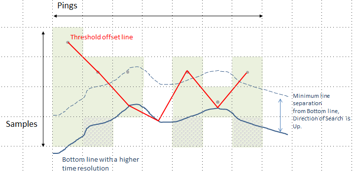
• The Threshold offset line has the same time resolution as the echogram. It is advised that the time resolution of Operand 1 and the line operand match. Otherwise, unwanted line time-mismatch artifacts may occur. See also Figure 2 Bottom line with a higher resolution than the echogram.
• Threshold offset operator settings.
• About the Threshold offset operator.

Illustrated examples

The following examples depict a stylized echogram with the following features:

• Eligible green samples =-40 dB = Vegetation
• White samples = -999 dB = Empty water
• Hatched samples represent ineligible samples for the Threshold offset algorithm.
• Boundary Threshold = -40 dB
• Grey dots represent the sample depth.

Figure 1 Time resolution of the Bottom line and the echogram match.

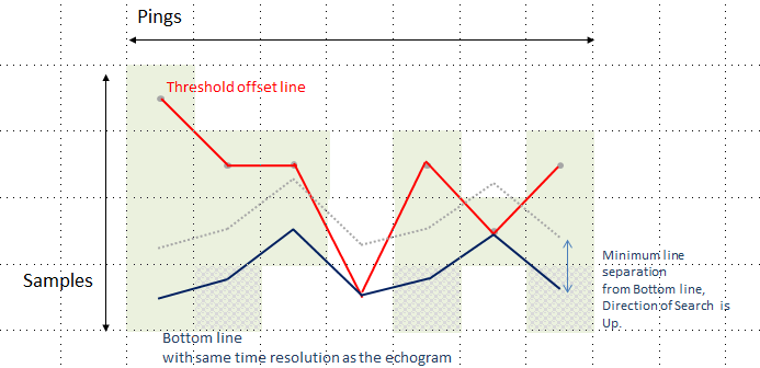
Figure 2 Bottom line with higher time resolution than the echogram

The Bottom line has a higher time resolution than the echogram. An unwanted artifact occurs when Threshold offset line dips below the Bottom line between ping 3 and 4.

Trained model bottom exclusion (experimental)

This utilizes the Trained model bitmap (experimental) operator with the "Bottom exclusion" Feature to detect setting to locate the bottom.

Then in the bitmap, starting from the Detection start range (m), it follows the following procedure for each ping in the input echogram. If you are recalculating the line, this applies to the bounding box of the selection instead.

The line pick supports the following data types for editable lines:

• Power
• Power pulse compressed
• Power wideband
• Sv
• Sv pulse compressed
• Sv wideband
• TS
• TS pulse compressed
• TS wideband
• Unspecified dB
  

Notes:

• The line pick for virtual lines only supports Sv data. Sv wideband data is currently unsupported.
• The model is trained with EK60 narrowband Sv data.

In the first step, Echoview determines the line status, and in the second step Echoview determines the line depth.

1. Count the number of contiguous ping sample strands comprising one or more true Boolean values.
1. If there are no such strands, it does not create a line segment.
2. If there is only a single contiguous fragment, it creates a line segment and assigns it a "Good" line status.
3. Otherwise, if there are multiple contiguous fragments, it creates a line segment and assigns it an "Unverified" line status.
2. Look up the Sv values (in the input echogram) for all the true samples in the bitmap.
1. It finds the highest Sv value and presumes this represents the bottom location.
2. From this sample the algorithm searches upwards until it reaches the first false sample.
3. It uses the depth of the 'final' true sample for the line segment it created in step 1.

Best bottom candidate

The bottom depth is picked for each ping in the context of surrounding pings. Nine settings can be entered under Single beam on the Lines and Surfaces page of the EV File Properties dialog box: Start depth (m), Stop depth (m), Minimum Sv for good pick (dB), Discrimination level (dB), Backstep range (m), Peak threshold (dB), Maximum dropouts (samples), Window radius and Minimum peak asymmetry.

The same settings can be entered on the Best bottom candidate line pick page of the Line Properties dialog box for a virtual line created with the Best bottom candidate line pick operator.

The Best bottom candidate algorithm assesses pings in groups referred to as ping contexts. In good data, the context is 64 pings wide, but if the bottom is not detected then the width is successively halved until either the bottom is found or the width has reached 8 without success.

The algorithm treats peaks in the ping data as candidates for the bottom echo. A peak is any contiguous series of samples with magnitude greater than the Peak threshold. Because the data contains noise, the definition of contiguous is relaxed by the Maximum dropout value. A peak can include any number of groups of samples below the Peak threshold, but the number of samples in any one group is less than or equal to Maximum dropout.

At various stages of the algorithm, the peak maximum and the Minimum peak asymmetry are considered. The rise side is defined as those samples closest to the transducer between the peak maximum and the Peak threshold. The decay side is defined by samples (in the same interval) on the other side of the peak maximum. Minimum peak asymmetry represents the ratio of the rise gradient to the decay gradient of the candidate peak. Candidate peaks that have a ratio less than the Minimum peak asymmetry are rejected.

From left to right, the diagrams above show:

• A ping (green line) in an echogram. The yellow rectangular region shows a context of pings. The echogram displays a series of echoes due to transducer ring down at the top, biomass in the water column and the bottom. On the left and right parts of the echogram, a bottom and two secondary bottoms (below the bottom) are displayed.
• The ping graph for the (green) ping. Samples are uniformly spaced in range. The green rectangle is centered on a candidate peak already found in the adjacent ping. The size of the search window is ± Window radius around the center of the search window.
• An expanded view of the search window (green rectangle of previous graph). The Peak threshold is shown as a blue line, the Discrimination level is shown as the dashed blue line. For this peak, if Maximum dropouts is set to 1, the algorithm would deem the candidate peak to be between and including the circled samples.

The algorithm works as follows:

1. The algorithm finds the first ping in the context that has more than one candidate peak. This is done by evaluating all the samples in the ping. The algorithm retains up to six of the highest peaks as candidates.
2. Each candidate peak is traced through the context using a search window. The aim is to find corresponding peaks in successive pings. If any part of a peak is found within the search window, that peak is considered. The highest peak in the search window is chosen. If no peak is found, the sample at the center of the window is used. The corresponding peaks found in successive pings form a candidate bottom series.
3. The values of the peak maxima are summed for each candidate bottom series. The series with the highest total wins. The winning series may not necessarily be the bottom as there may be no bottom.
4. The algorithm maintains a level of confidence in its detection. The magnitude of this confidence, and its sign, are used to modify detection behavior. Confidence is expressed as the number of contiguous pings from which the bottom has been found. If the chosen bottom series sinks below the lower edge of the data, the magnitude of confidence is maintained but its sign becomes negative. In this case, the algorithm is confident that from here on there is no bottom in the data. Negative confidence is used to dismiss series that appear suddenly in the water column. If a series is detected rising from the lower edge of the data, it is accepted as the bottom.
   • One consequence of this approach is that the result for a selection may differ from the result of considering the whole echogram. This is because a selection starts with zero confidence.
5. If the bottom is not continuous between contexts, and the detected bottom is close to the lower edge of the data, then the end of the context is reassessed, ping by ping, to find the point where the bottom crosses the lower edge of the data.
6. The final step is to use the Discrimination level and Backstep range settings to position the bottom line above the bottom signal. For each ping, the algorithm steps back from the peak maximum towards the transducer until the signal sinks below the Discrimination level. The Backstep range is subtracted from the range at which the peak crosses the Discrimination level.

Note: The algorithm applies itself to samples inside the rectangular bounding box for parallelogram and polygon selections and then returns a pick for the selection shape (only).

The default settings are:

Setting	Default value
Start depth	5 m
Stop depth	1000 m
Minimum Sv for a good pick	-70 dB re m-1
Use Backstep	Checked
Discrimination level	-50 dB re m-1
Backstep* range	0.00 m
Peak threshold	-50 dB re m-1
Maximum dropouts	2 samples
Window radius	8 samples
Minimum peak asymmetry	-1

See About the Best bottom candidate line pick and Best bottom candidate settings for more information.

Maximum SV

This algorithm picks the bottom as the depth of the sample with the strongest backscattering strength (Sv). If the Sv of the bottom sample is greater than or equal to the Minimum Sv for good pick value then the bottom pick is given status of good, otherwise it is given a status of bad. It searches between a specified Start depth and Stop depth only.

Three settings can be entered under Single beam on the Lines and Surfaces page of the EV File Properties dialog box: Minimum Sv for good pick (dB), Discrimination level (dB) and an optional Backstep range (m).

The same settings can be entered on the Maximum Sv line pick page of the Line properties dialog box for a virtual line created with the Maximum Sv line pick operator.

The algorithm works as follows:

1. Search within the depth limits of the current selection (or the specified start depth and stop depth) to find the sample with maximum backscattering strength (Sv).
2. Search up the ping starting at the maximum sample to find the first sample whose Sv is less than Discrimination Level. This occurs below point 2 in the diagram below.
   
   If the sample just below the Discrimination Level is a no data sample, then the depth is the  depth of the sample just above the Discrimination Level.
   Otherwise, the depth is at the Discrimination Level. This is determined as the linear interpolation (for depth) of the samples just below and just above the Discrimination Level.
3. The depth of the pick for the ping is the depth found in step 2 less the value of the Backstep range.
4. If the Sv of the sample picked in step 1 is greater than or equal to the Minimum Sv for good pick then give the bottom pick a status of good, otherwise give it a status of bad.

Notes:

• The resultant picked value is the one evaluated in step 3. If you require the picked line to be below X meters, then the Start Depth should be X + Backstep range.
• Step 2 was modified in Echoview 4.30. Editable lines picked before Echoview 4.30 will not change but these lines will be different from lines picked (on the same data) with Echoview 4.30. Virtual lines created using the Maximum Sv algorithm, from Echoview 4.20, will change. Such virtual lines will be picked using the algorithm implemented in Echoview 4.30.
• The difference between the two versions of the Maximum Sv algorithm is that the earlier version returns a picked line that is deeper by one to two samples for a Backstep range of 0m.
• The algorithm applies itself to the samples inside parallelogram or polygon selections and can return a pick even if there is no bottom in some sections of the selection.

The algorithm is illustrated on a sample graph of Sv values as follows:

• Point 1 illustrates the range of the pick when Backstep is unchecked.
• Point 3 defines the range of the pick when Backstep is checked and a Backstep range is specified.

The default settings are:

Setting	Default value
Start depth	0 m
Stop depth	1000 m
Minimum Sv for good pick	-70 dB re m-1
Use Backstep	Checked
Discrimination Level	-50 dB re m-1
Backstep* range	0.00 m

Delta Sv

This algorithm examines only the change in Sv over one pair of neighboring samples at a time and returns the range of the nearest sample which is detected after a rise of “Delta Sv” dB which is greater than the specified minimum. It searches between a specified Start depth and Stop depth only.

Note: The Delta Sv bottom pick algorithm was designed for a specific dataset of EchoListener files, and is not recommended for general use.

The default settings are:

Setting	Default value
Start depth	0 m
Stop depth	1000 m
Minimum Sv for good pick	15 dB re m-1

See also

Line picking
Single beam (line pick) on the Lines and Surfaces page
Multibeam bottom detection algorithm
About the Best bottom candidate line pick
About the Threshold offset operator