Configuring a bottom classification

Echoview bottom classification is suitable for a single beam Sv variable with a first bottom echo, or single beam Sv variable with a first and second bottom echo. It is advisable to prepare Sv echogram data so that the classification algorithms are applied to acceptable Sv data. Preparation may involve identifying and dealing with unsuitable echogram data (noise, bad samples, unwanted data etc).

The Bottom classification algorithms are applied when you use:

Sv echogram > Echogram menu > Classify Bottom
- OR -
Dataflow window > Bottom points variable > Shortcut menu > Reclassify Bottom
- OR -
Vertical selection > Shortcut menu > Classify Bottom (See also Vertical selection note.)

The Classify Bottom feature requires the configuration of the settings specific to the Sv variable and settings specific to the bottom classification algorithms.

Sv Variable settings
EV File Properties settings
Tips

Sv Variable Properties

Bottom line

A bottom line is important because it delineates the echo from the bottom from echoes in the water column. The bottom line and the echoes below that line are where Echoview applies bottom classification algorithms.

Create an editable line using a line pick algorithm. To ensure that echoes from the water column are excluded, the line pick may require manual editing.

Bottom echo threshold at 1 m (dB)

The ping graph, depicted below, is a stylized representation of the first and second bottom echoes. Annotations for important features that are used as variable settings include: Bottom line depth (at the ping) and Bottom echo threshold at 1m. The start point for first echo integration calculations represents the extra distance the beam travels in order for a complete acoustic pulse (for the whole beam) to travel in the substrate. This point is not an explicit setting, rather it is an inherent characteristic of the beam geometry. (See also The beam and seabed diagram).

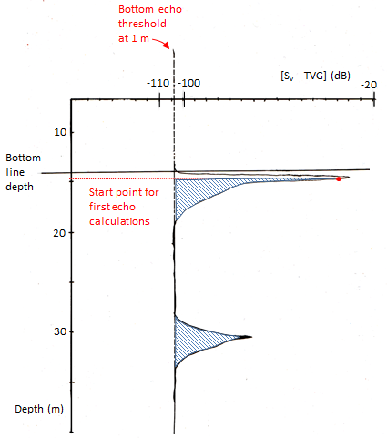
Ping graph for bottom classification

Figure 1: Ping graph: Sv - TVG (dB) versus Depth (m).

A Bottom echo threshold at 1m (dB) represents the Sv value that estimates the end of the first echo. Echoview identifies three consecutive samples that are under the threshold value. The first of the values is deemed to be the end of the first echo.

There are two ways to estimate the Bottom echo threshold value.

Ping graph

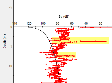
Use an Sv ping graph to display an Sv TVG Curve. The graph shows (highlighted) peaks for the first and second bottom. It also shows the TVG.

Pingr graph

Figure 2: Ping graph: Sv versus Depth, and Sv TVG Curve.

Data generator

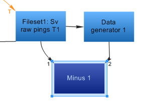
Figure 3: Dataflow operators to remove TVG from the Sv variable.

Similarly, a ping graph for the virtual variable representing the Sv variable minus the Data Generator (operand Sv variable, algorithm TVG curve) can remove the TVG from the Sv variable and make it easier to estimate the Sv value for the end of the first bottom echo.

Background noise removal variable

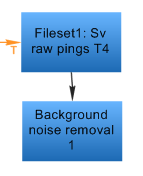
An alternative way to estimate the Bottom echo threshold at 1m (dB) uses the Background noise removal operator.

Use the Sv variable as the input operand to the Background noise removal operator. On the Background removal operator set Bottom echo threshold at 1m (dB) to a value of -500 dB and run Classify Bottom on the Background noise removal variable.

Note that the Background noise removal operator takes time to generate its virtual variable data. So it is a good idea to scroll through the virtual echogram before running a bottom classification.

The advantage with this approach is that background noise is removed from the Sv data and you can take the guess work out of the estimate for Bottom echo threshold at 1m (dB) by using the fact that the Background noise removal operator sets identified noise samples to -999 dB. Using -500 dB as a Bottom echo threshold ensures that Echoview includes all samples in the echo but excludes samples that are or close to the noise.

Background noise estimate

Figure 4: Dataflow with the Background noise removal operator.

Depth normalization reference depth

A bottom echo encodes time and energy information for one transmitted pulse incident on the bottom substrate. For a normal incidence single beam the transmitted pulse travels a distance of cτ /2. However, at the off-axis part of the beam the same pulse travels a distance greater than cτ/2. As a result, the bottom echo extends over this Effective pulse length. c is the speed of sound in water (m/s) and τ is the transmitted pulse duration (s).

A Depth normalization reference depth specifies a reference depth used to normalize pulse length. The best value for the reference depth is the average depth of the bottom, which may be estimated with bottom line data from a table or graph.

The exaggerated diagram illustrates the beam geometry, shows how the effective pulse length changes with depth and the reason for the Off axis angle offset. When calculating the roughness index, Echoview begins calculations from the depth given by Bottom line depth plus the distance of cτ /2 plus the off-axis angle offset. See also Depth normalization algorithms.

Beam_spread_geometry

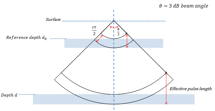
Figure 5: The beam and effective pulse length at different depths.

Bottom classification integram

It is useful to view echogram data in relation to bottom points displayed in the integram area. For a to-be-created bottom variable this can be done by selecting Show bottom classes on integram on the Classify Bottom dialog box. To change the bottom points variable displayed in the integram specify a different data source with the Bottom variable list under the Integram section of the Echogram Display page of the Variable Properties dialog box.

Other settings

Analysis page Exclusion lines are ignored by bottom classification. See also Integration Results note.

Analysis page Analysis bad data settings are unsuitable for bottom classification and may result in a meaningless bottom classification.

Classify Bottom EV File Properties

The Bottom Classification page of the EV File Properties dialog box offers settings for the feature extraction interval, first and second bottom features, principal component dimensions, clustering algorithms and iterations for clustering. Second bottom features (Bottom_hardness_normalized and Second_bottom_length_normalized) may be calculated only when a second bottom echo exists.

For a detailed discussion of the algorithms and algorithm limitations refer to Bottom classification algorithms.

Tips

Dataflow window > Bottom points variable > Shortcut menu > Reclassify Bottom can reuse features and generally has a shorter processing time. However, the previous Bottom points in the variable are overwritten.
Use Bottom Class Allocation Manual and Class count, and increase Clustering iterations when you are have a better feel about the number substrates in the data. An increase in Clustering iterations increases the processing time.
Automatic PCA may find up to five principal components. Follow with automatic clustering using both algorithms to produce classes that give a general feel for the data. Then try specific component dimensions and a manual class number with increased cluster iterations to fine tune the classification. From a physical perspective, features that are likely to be strong component dimensions include: Roughness index, Hardness index and (first) bottom rise time. Previous or other substrate information may help with the selection of class number. Bottom points graphs of features may also help in identifying trends in the data. See also Examples for k in lake data.
A bottom classification may include unclassified points that are assigned a no data value.