dB difference Absolute
You can use concurrently recorded multiple frequency data and dB difference techniques to differentiate the mean volume back scatter of species. Several discussions appear in Simmonds and MacLennan17, 18 (2005) and work on the subject can be found in papers by Mitson et al19 (1996), Kang et al20 (2002) and Korneliussen and Ona21 (2003).
The basic idea is that target strength is dependent on frequency in different ways for different species. Two species of scatterers (e.g. fish and zooplankton) may have different mean backscattering strengths at different frequencies. Since the difference is in the mean backscatter it is usual to average the backscatter in cells or regions prior to calculating the dB difference.
This idea is applied to multiple frequencies allows a better definition of the frequency response for the classification.
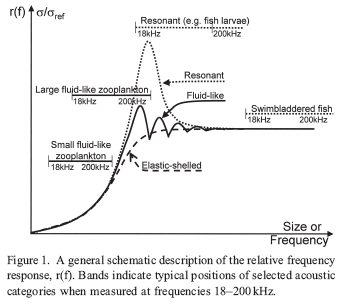
Screenshot displays the hydroacoustic frequency response of fish and zooplankton from Korneliussen and Ona21.
When you use dB difference techniques, obtaining unbiased measurements requires high signal-to-noise ratio at multiple frequencies. Therefore you need to avoid the integration of noise even for one frequency. As a consequence the technique is limited to the range at which the highest frequency has a good SNR. Refer to De Robertis and Higginbottom22 (2007) for an approach to this subject.
The following technique description implements a number of processing stages:
- Remove samples below acoustic bottom and above surface noise layer.
- Echo integrate (resample) the two variables.
- Calculate the “dB difference” between the two resampled variables.
- Select those data which meet a specified criterion of “dB difference”.
- Integrate the resultant data set by cells.
Virtual variables create a “dB difference” echogram and then classify areas of the original echogram according to specified dB difference criteria. The technique outlined is not necessarily complete or applicable to any particular species classification task. You are referred to the scientific literature for working examples of this type of analysis.
Scenario
|
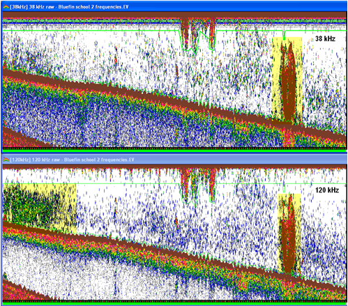
Screenshot shows Sv echograms of EK60 data from a 38 kHz and a 120 kHz transceiver. The color display minimum is -90dB for both echograms. The highlighted areas show an aggregation on the RHS in the 38 and 120 kHz echograms and an aggregation on the LHS on the 120 kHz echogram. It is visually obvious that the shallow aggregation has a stronger frequency response at 120 kHz. You would also be able to see this behavior using the Frequency response graph (View men >, Graph Frequency response). |
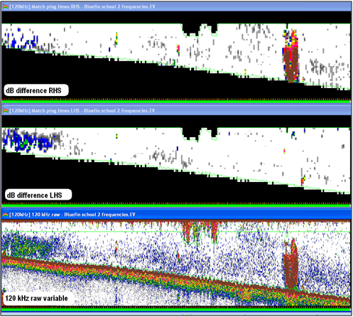
Screenshot shows dB difference echograms and the 120 kHz raw variable. |
Dataflow
|
Dataflow object |
Aim |
Echoview feature |
|
38 kHz raw, 120 kHz raw |
Sv data for 38 kHz transducer. Sv data for 120 kHz transducer. |
Raw variable |
|
38 kHz cleaned, 120 kHz cleaned |
Apply the line and bad data region exclusion settings specified on the Analysis page of the Variable Properties dialog for its input variable, changing excluded data points to 'no data' values. Use the Processed data operator. Input variable is a raw variable. Typical lines can be:
|
|
|
38 kHz resampled, 120 kHz resampled |
Create variables with the same ping geometry and with reduced number of samples (to speed up computation). Set up the required ping geometry with the Resample by number of pings operator. The original ping geometry of the raw variable can be viewed using Shortcut menu > Show Information > Ping tab. Use the Resample by pings operator. One input variable is 38 kHz cleaned. The other input variable is 120 kHz cleaned. Resample operator settings:
|
|
| dB difference (120-38) |
Evaluate the dB difference 120 kHz data - 38 kHz data. Use the Minus operator. Operand 1 = 120 kHz resampled Operand 2 = 38 kHz resampled |
Minus operator |
| Range mask for LHS aggregation |
Create a bitmap to dictate which LHS samples to retain. Use the Data range bitmap operator. The input variable is dB difference (120 - 38). The operation sets a "true" value for each input value that is within a specified range, and a "false" value for each input value that is outside the specified range. "No data" values are always translated to "false". Minimum in-range value Maximum in-range value The in-range values were optimized by visual inspection of the Range mask echogram and later on with the final echogram for the LHS. You want to isolate the LHS aggregation. |
Data range bitmap operator |
| Range mask for RHS aggregation |
Create a bitmap to dictate which RHS samples to retain. Use the Data range bitmap operator. The input variable is dB difference (120 - 38). The operation sets a "true" value for each input value that is within a specified range, and a "false" value for each input value that is outside the specified range. "No data" values are always translated to "false". Minimum in-range value Maximum in-range value The in-range values were optimized by visual inspection of the Range mask echogram and later on with the final echogram for the RHS. You want to isolate the RHS aggregation. |
Data range bitmap operator |
| 120 kHz classified by dB difference with mask for LHS |
Create a mask to apply the dB difference (120 -38) classification. Use the Mask operator. Operand 1 = 120 kHz resampled Operand 2 = Range mask for LHS aggregation |
Mask |
| 120 kHz classified by dB difference with mask for RHS |
Create a mask to apply the dB difference (120 -38) classification. Use the Mask operator. Operand 1 = 120 kHz resampled Operand 2 = Range mask for RHS aggregation |
Mask |
|
Resample vertically LHS Resample vertically RHS |
Return to the ping geometry of raw variable. This pair of steps (Resample vertically and Match ping times) approximates the ping geometry of the 120 kHz raw variable – to facilitate visual comparison for the dB difference results. Set up the required ping geometry with the Resample by number of pings operator. The original ping geometry of the raw variable can be viewed using Shortcut menu > Show Information > Ping tab. Input variable is 120 kHz classified by dB difference with mask for LHS. The other input variable is 120 kHz classified by dB difference with mask for RHS. Resample operator settings:
|
Resample by number of pings |
| Match ping time LHS |
Return to the ping geometry of raw variable. This pair of steps (Resample vertically and Match ping times) approximates the ping geometry of the 120 kHz raw variable – to facilitate visual comparison for the dB difference results. Use the Match ping times operator. Operand 1 = Resample vertically LHS Operand 2 = 120 kHz raw Allowed (slop) = 600 seconds |
Match ping times |
| Match ping time LHS |
Return to the ping geometry of raw variable. This pair of steps (Resample vertically and Match ping times) approximates the ping geometry of the 120 kHz raw variable – to facilitate visual comparison for the dB difference results. Use the Match ping times operator. Operand 1 = Resample vertically RHS Operand 2 = 120 kHz raw Allowed (slop) = 600 seconds |
Match ping times |
References
| 17 | Simmonds J. and MacLennan D. (2005) Fisheries Acoustics: Theory and Practice. Second edition, Blackwell Science. Fish and Aquatic Resources Series 10. (ISBN-10: 0-632-05994-X, ISBN-13: 978-0-632-05994-2). p262, Chapter 7 Plankton and Micronekton Acoustics. |
| 18 | Simmonds J. and MacLennan D. (2005) Fisheries Acoustics: Theory and Practice. Second edition, Blackwell Science. Fish and Aquatic Resources Series 10. (ISBN-10: 0-632-05994-X, ISBN-13: 978-0-632-05994-2). p334-336. |
| 19 | Mitson R.B., Simard Y. and Goss C. (1996) Use of a two-frequency algorithm to determine size and abundance of plankton in three widely spaced locations. ICES Journal of Marine Science, p53: 209-215. |
| 20 | Kang, M., Furusawa, M., and Miyashita, K. (2002). Effective and accurate use of difference in mean volume backscattering strength to identify fish and plankton. ICES Journal of Marine Science, p59: 794–804. |
| 21 | Korneliussen, R. J., and Ona, E. (2003). Synthetic echograms generated from the relative frequency response. ICES Journal of Marine Science, p60: 636–640. |
| 22 | De Robertis, A., and Higginbottom, I. (2007). A post-processing technique to estimate the signal-to-noise ratio and remove echosounder background noise. ICES Journal of Marine Science, 64: p1282–1291. |