Bottom classification algorithms

The Bottom classification algorithms are applied when you use:

• Sv echogram > Echogram menu > Classify Bottom
• - OR -
• Dataflow window > Bottom points variable > Shortcut menu > Reclassify Bottom
• - OR -
• Vertical selection > Shortcut menu > Classify Bottom

Note: The bottom points for a vertical selection bottom classification are valid within the selection boundary. The first and last bottom points of this type of classification should be disregarded, as they are an artifact of the time buffer used to ensure the validity of bottom points within the selection.

Background

Echoview bottom classification algorithms are based on useful research findings from papers and reports. The reports by Hamilton (2001) and Anderson et al (2007) provide comprehensive introductions to and offer an extensive review of background theory, systems, algorithms, system strengths, system weaknesses and future directions. See also Bottom classification - practical notes.

Algorithm summary

• Feature extraction interval
• Bottom features
• Principal component analysis - cluster dimensions
• k-Means clustering
• Examples for k in lake data
• Bottom classification notes
• Footnotes

The Classify Bottom process applies bottom classification algorithms to pre-configured single beam Sv echogram data. Normal incidence, single beam Sv data is used because:

• Sv is normalized to a reference volume (dB re 1 m2/m3)
• single beam transducers may be reliably calibrated with an acoustic sphere prior to data collection
• Sv data is corrected for acoustic absorption and spreading (TVG is commonly applied)
• normal incidence offers the simplest and strongest echo. Anderson et al1 suggests that bottom slopes be restricted to less than half a beam width. This is small enough to ensure that normal incidence reflection continues to be valid and that the echo shape is information rich. With steep slopes, echo amplitude reduces and echo shape becomes information poor. "...Sediments in areas with slopes more than about a half beam width cannot be classified acoustically in the same manner as flatter regions (von Szalay and McConnoughey, 2002). It is often possible to separate them into a “slope” class, which may be adequate if it is known that only particular sediments, bedrock perhaps, are stable with these slopes. These observations apply also to ship roll and, less commonly, pitch."
• Figure 1 depicts Figure 4.2 from Anderson et al, it shows a stylized depiction of a single beam sonar insonifying a flat horizontal seabed and a flat sloping seabed of the same substrate type. The graphs of the tail of the first echo integration (E1) with times t1, t2, t3 and t4 model the error encountered when the bottom slopes.
  
  
• 
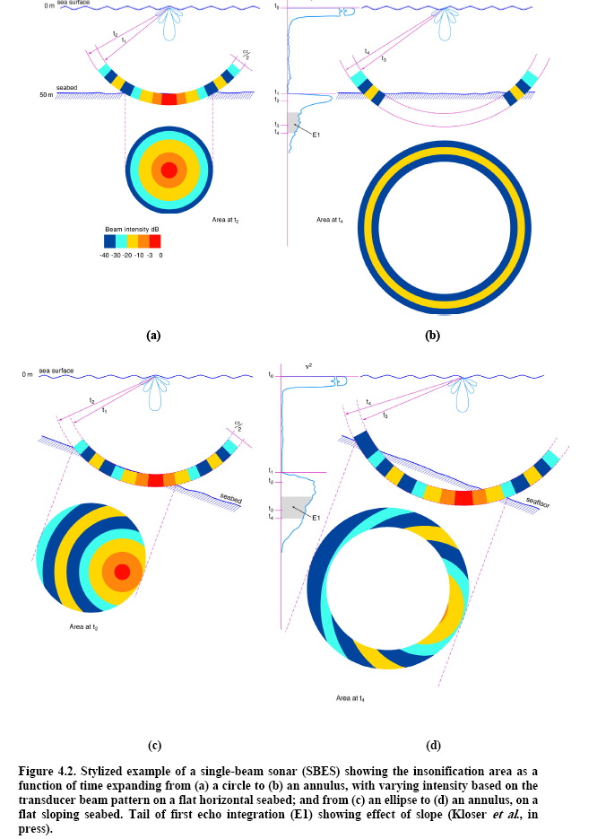
• Figure 1 depicts Figure 4.2 from Anderson et al.

A single beam transducer may be calibrated with an acoustic sphere. This ensures the collection of quantitative backscatter data. Quantitative data together with restrictions on beam incidence and bottom slope make it possible to achieve repeatable bottom classifications of a substrate.

Feature extraction interval

A bottom feature represents a measured aspect of the first or second bottom echo. Bottom features are calculated for each feature extraction interval. The feature extraction interval aims to use an average of similar echoes to get better stability in the data for a classification. The feature interval is affected by ping rate, ping foot print (beam width and seabed depth) and vessel speed. The Echoview default value is ten pings. This value is used by Siwabessy2 and is discussed by Hamilton3. Anderson et al4 noted that a fifteen ping average minimizes the measurement variability in a 38 kHz single beam echosounder system. Eillingsen et al5 used five pings for their 50 kHz sounder. The minimum size for a feature extraction interval is three valid pings. For intervals with an even ping number, the bottom point time, latitude, longitude, depth and altitude is the interpolation of the interval's middle ping times etc. Principal component analysis times can be sensitive to the size of the feature extraction interval.

Bottom features

First echo

• Bottom_roughness_normalized (dB re 1m2/m3)
• First_bottom_length_normalized (m)
• Bottom_rise_time_normalized (m)
• Bottom_line_depth_mean (m)
• Bottom_max_Sv (dB re 1m2/m3)
• Bottom_kurtosis (unitless)
• Bottom_skewness (unitless)

Second bottom echo

• Bottom_hardness_normalized (dB re 1m2/m3)
• Second_bottom_length_normalized (m)

Extent of the first and second bottom echoes

• Bottom line depth is a reference point for the detection of valid first and second bottom echoes. A valid bottom echo needs:
  1. Three consecutive sample values above -60 dB.
  2. Then three consecutive sample values below the Analysis page setting Bottom echo threshold at 1 m (dB).
• Bottom echo threshold at 1 m (dB) is used to determine the end of the first bottom and second bottom echo. The first of the three consecutive samples below Bottom echo threshold at 1m (dB) is the end of a valid bottom echo.
• The start point for the calculation of Bottom_roughness is given by Bottom line depth plus the distance of cτ /2 plus the off-axis angle offset. The offset accounts for the extra distance the complete pulse has to travel in the substrate (Anderson6).
• When present, the second bottom echo starts at twice the depth of the first bottom echo (Anderson7). Echoview's implementation considers the transducer draft and orientation and the Z coordinate of the water level and uses twice the bottom line depth for the start of the second bottom echo.
• The whole of the second bottom echo is used for the calculation of Bottom_hardness.

Notes:

• See also: Bottom classification ping graph.
• A bottom classification is not run if PCA is selected and any of the features (selected in the Feature Extraction list) are no_data for every interval.
• First bottom echo features are dependent on the quality of the Bottom line. Incursions of the bottom line into the first bottom echo can lead to indefinable first bottom echo features. To a lesser extent, a poor Bottom line may affect second bottom features.
• When Bottom echo threshold at 1 m (dB) is set too high or too low, the condition for three samples below that threshold may not be satisfied for the echo and hence a valid bottom point can't be determined. Where this occurs for all Feature intervals, a message is sent to the Message dialog box. A classification may be more successful when Bottom echo threshold at 1 (m) is estimated through a background noise removal variable method.

Depth normalization reference depth algorithms

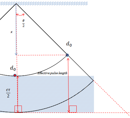
Figure 2: The geometry of the beam, showing the off-axis angle offset distance and the differences in pulse length. An associated annotated diagram is discussed under Configuring a bottom classification: Depth normalization reference depth.

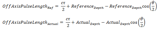
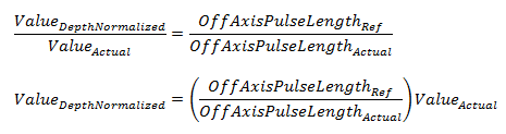
Some bottom features are depth normalized to account for variations in pulse length with depth. Considering the geometry of the beam, the expression for the total distance that the off-axis part of the beam needs to travel one whole pulse length in the substrate is: We can define these OffAxisPulseLength equations: We can also use this relationship:

Where:

c	=	Speed (m/s) of sound in the medium.
τ	=	Pulse length (s) of the transducer.
θ	=	Major-axis 3dB beam angle of the transducer.
d0	=	Normal incidence start depth (m) of the first bottom echo at ping p.
OffAxisPulseLengthRef	=	Off-axis pulse length where the normal incidence start depth is specified by the Depth normalization reference depth.
ReferenceDepth	=	The Depth normalization reference depth specified under Bottom settings on the Analysis page of the Variable Properties dialog box.
OffAxisPulseLengthActual	=	The Off-axis pulse length of the first bottom echo, where the normal incidence start depth of the first bottom echo is given by ActualDepth for ping p.
ActualDepth	=	The depth of the Bottom line (at normal incidence) for the first bottom echo at ping p.
ValueDepthNormalized	=	The depth normalized bottom feature, where Value is: Bottom_roughness Bottom_hardness First_bottom_length Second_bottom_length_bottom Bottom_rise_time
ValueActual	=	The bottom feature, where Value is: Bottom_roughness Bottom_hardness First_bottom_length Second_bottom_length Bottom_rise_time

Echoview determines one bottom point per feature extraction interval. At this stage, bottom point data includes time, latitude, longitude, depth, bottom features. Each bottom feature is a mean of the measured ping characteristics in the feature interval.

Principal component analysis - cluster dimensions

The next processing stage calculates the normal deviate (Z-score) for bottom features from the feature extraction intervals in the echogram data. Unitless, statistical feature values are processed by the statistical procedure of Principal Component Analysis (PCA) followed by k-Means clustering. PCA and k-Means clustering have been used successfully with field data by a number of seabed classification researchers. The data mining literature cites advantages and disadvantages of each algorithm and of the pairing of the algorithms.

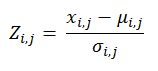
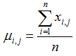
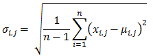
Normal deviate algorithm:

where:

Zi, j	=	Normal deviate for bottom feature i in the echogram set j
x i,j	=	Bottom feature value i in the echogram set j
μi,j	=	Mean of the bottom feature in the echogram set j, where n is the number of bottom feature i in the set j.
σi,j	=	Corrected sample standard deviation of the bottom feature in the echogram set j

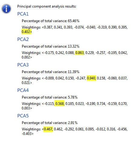
Principal component analysis is a statistical technique that explores the underlying structure in a data set. The technique identifies principal components by calculating the largest variations of the dimensions in the data set. Under bottom classification, bottom features are the dimensions of the data set. PCA determines the principal components as cluster dimensions of the data.

Siwabessy et al (2000) offer a clear discussion about the usefulness of PCA: "... To reduce the dimensionality of the acoustic data, Principal Component Analysis (PCA) was applied... PCA is in general a data transformation technique. It attempts to reduce the dimensionality of a data set formed by a large number of interrelated variables but retains sample variation (information) in the data as much as possible. The process includes an orthogonal transformation from the axes representing the original variables into a new set of axes called principal components (PCs). The new axes or the PCs are uncorrelated one to another and are ordered in such a way that the first few PCs hold as much of the total variation as possible from all the original variables. While PCs from the geometric point of view are orthogonal projections of all the original variables, PCs algebraically are linear combinations of the original variables. ..."

Automatic PCA uses matrix mathematics and eigen vectors to determine five cluster dimensions. Where the cluster dimensions are user specified, only three cluster dimensions are available. Legendre et al (2002), in their study of QTC data, comment on the percentage variance in a data set that can be covered by a number of Principal Component dimensions (PCs): one data set had three PCs accounting for 96.2% and seven PC for 99.2% while another data set had 3-5 PCs for 95% and 6-10 PCs for 99%.

With reference to Figure 3, weightings follow the feature order on the Bottom classification page of the EV File Properties dialog box. Highlighted weightings show the dominant feature. PCA1 is First bottom skewness PCA2 is Second bottom length normalized PCA3 is (first) Bottom rise time normalized PCA4 is Bottom hardness normalized PCA5 is Bottom roughness normalized

Figure 3: A screen shot of an Automatic PCA message sent to the Messages dialog box.

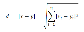
Echoview uses cluster dimensions to characterize each bottom point in cluster dimension space. A bottom point with five cluster dimensions would have coordinates of (a, b, c, d, e), while a bottom point with three cluster dimensions would have coordinates (g, h, i). The distance between two points x and y in a Euclidean Rn space9 and therefore of two bottom points in n-dimension cluster space is given by:

Note: The algorithms for automatic PCA are iterative and contain tests for the validity of the resulting eigenvectors. Automatic PCA uses a fixed number of iterations and if the eigenvectors fail to resolve in the allowed time, the algorithm stops and a message is sent to the Messages dialog box. Using a smaller Feature extraction interval may fix this problem.

k-Means clustering

The last stage of the bottom classification uses k-Means algorithms to cluster bottom points into classes. Generally, "the k-Means algorithm aims to partition n observations into k clusters in which each observation belongs with the cluster with the nearest mean"8. Choosing the bottom points for the center of clusters and allocating bottom points to clusters is carried out by an initialization algorithm modeled on the k -Means++ technique.

The initialization algorithm does the following:

1. Choose the first cluster center at random from among the bottom points.
2. For each data point x, compute D(x), the distance between x and the nearest center that has already been chosen.
3. Of the ten percent of bottom points farthest away from the previous center point, choose a random bottom point for the next center point.
4. Repeat Steps 2 and 3 until k* centers have been chosen.
5. Now that the initial cluster centers have been chosen, proceed using the selected k-Means clustering method.

Notes:

• *Under the Bottom Class Allocation Manual setting, the Class count specified by the user is used for k. Under the Automatic setting, the initial k value is 20.
• To improve computational performance, distance squared is used by k-Means algorithms.
• Elkan (2003) triangle inequality methods are used to accelerate k-Means algorithms.

After the initialization of cluster center points, the k-Means algorithms (under Manual or Automatic setting) allocate bottom points to clusters in such a way that the cluster variance is minimized. The value for Clustering iterations controls how many times the allocation/minimization process is applied to the set of bottom points. In Automatic clustering messages, an Iteration run is referred to as K-number #.

In Echoview, the final value of k defines the number of bottom classes. k can be specified using the Manual, Class count setting. A WCSS algorithm is used to optimize the points assigned to clusters. WCSS is the acronym for "within cluster sum of squares" which is a measure of the compactness of a cluster. Under the Manual scenario, an estimate for k may be based on substrate sampling, other sources of ecological/geographical/environmental knowledge or an assessment of the probable value from clustering sensitivity analysis.

When you can't estimate k, the clustering algorithm offers methods to identify k. One method is the WCSS with elbow method. A WCSS algorithm is used to optimize the points assigned to clusters. The ratio of the within-group-variance to the maximum-within-group-variance is calculated for successive cluster numbers. This data when graphed often approaches a steady value after an "elbow value". The WSCC with elbow method outputs the "elbow value" as the estimate of the number of bottom classes. Under the Automatic setting, ratio and cluster number information is sent to the Messages dialog box.

Another method to identify k is to use the Calinski-Harabasz (1974) criterion "which is suited for k-Means clustering solutions with squared Euclidean distances". The optimal number of clusters is the solution with the highest Calinski-Harabasz index value"10. Legendre et al (2002) noted that a simulation study by Milligan and Cooper (1985)10 of k criteria used for cluster analysis found that the best criterion in the "least-squares sense" was the Calinski-Harabasz criterion. Under the Automatic setting, ratio and cluster number information is sent to the Messages dialog box.

Examples for k in lake data

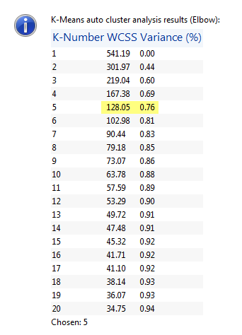
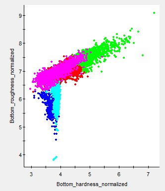
Figure 4: Screen shot of Elbow method message sent to the Messages dialog box. The "elbow value" is highlighted. This classification includes features of the first and second bottom echoes and is run on survey data from Scott Lake. Seven thousand bottom points are classed. Figure 6: Graph of Elbow classes for the bottom classification message from Figure 3. This graph plots the relationship between two dimensions. Automatic PCA outputs five cluster dimensions which may display other relationships.

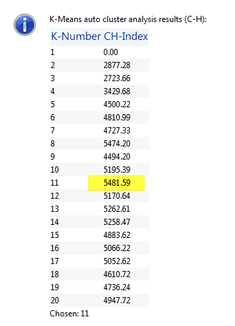
Figure 5: Screen shot of Calinksi-Harabasz message sent to the Messages dialog box. The "highest value" is highlighted. This classification includes features of the first and second bottom echoes and is run on survey data from Scott Lake. Seven thousand bottom points are classed. Figure 7: Graph of CH classes for the bottom classification message from Figure 4. This graph plots the relationship between two dimensions. Automatic PCA outputs five cluster dimensions which may display other relationships.

Figure 8: An Echoview bottom classification run on the (same) Scott Lake data. Seven thousand bottom points are classed using three cluster dimensions (Roughness_normalized, Hardness_normalized, Bottom rise time normalized) and a Manual Class count of 14. Class information was drawn from completed substrate grabs and video studies of Scott Lake. The classification has been constrained to three cluster dimensions, that were picked because they are likely to be dominant in both the theoretical and physical sense. This Scott lake manual classification offers clustering that fits more easily with known information about the survey area than the purely mathematical solutions offered by an automatic PCA with Elbow or Calinski-Harabasz estimate for k. Many thanks to Milne Technologies for permission to use its Scott lake data.

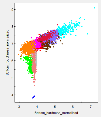
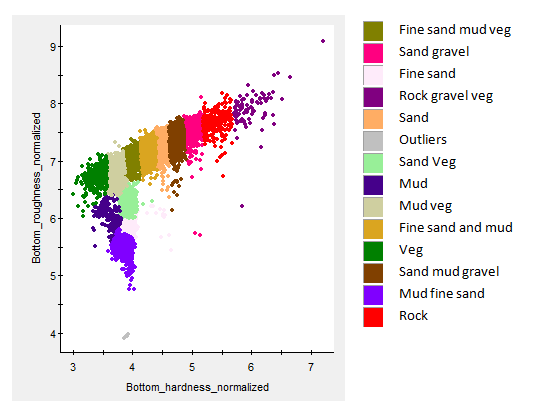
After a classification is complete, a bottom points variable appears in the Dataflow window. Bottom feature data may be analyzed on graphs, a table and as exported data. Bottom classes may be analyzed on graphs, a table, in the integram, on a bottom points cruise track and as exported data. Under the table, bottom class may be edited.

Bottom classification notes

• The clustering of multivariate data is a difficult problem. Purely mathematical solutions can be non-unique due to local minima/maxima in the data and the k-Means++ random initialization of cluster centers. A mathematical solution may even display a mismatch to the realities (or contexts) of the data. Legendre et al (2002) noted this effect with the Calinski-Harabasz criterion in some data sets (unpublished, pers. comm. Hewitt et al NIWA).
• Automatic clustering runs calculations for 20 clusters and outputs the main method values to the Message dialog box.
• When a bottom classification feature can't be calculated, a no data value is recorded and the bottom point is handled as Unclassified.

Footnotes

1. p39 (Anderson 2007)
2. 38 kHz, 200 kHz sounders (Siwabessy et al, 2004)
3. DSTO-TN-0401 3.13 Averaging returns (Hamilton)
4. p77 (Anderson 2007)
5. Ellingsen et al 2002
6. p75, Figure 4.1, Figure 4.2 (Anderson 2007)
7. p40 (Anderson 2007)
8. https://en.wikipedia.org/wiki/K-means_clustering
9. Weinstien, E. W. MathWorld
10. Mathworks: Calinski-Harabasz criterion and Calinski and Harabasz (1974).

See also

About bottom classification
Configuring a bottom classification
Bottom classification analysis options
Bottom classification - practical notes