School Detection module algorithms
This page covers school detection algorithms applied to single beam, split beam, and dual beam data only. 3D school detection uses an entirely different school detection algorithm.
A detected school is defined as an analysis region in Echoview. The only difference between regions created with the School Detection module and other regions is that the region boundaries of "schools" are constrained to follow the boundaries of data points. That is, in the depth-time space of an echogram, the rectangle that a data point is considered to occupy - having a thickness equal to the sample thickness and a width equal to that of the ping (which is equal to half the time since the previous ping plus half the time to the next ping). Note that regions are defined in terms of depth and time (see About regions).
A restriction in the School Detection module, requires that any single detected school spans a part of the echogram with constant vertical resolution (that is, the sample thickness remains unchanged over the interval of detection). If the sample thickness changes in the middle of a visible school, Echoview will generate one region for each range of pings with constant sample thickness.
In some cases, such as for corrected lengths and thickness, there are restrictions on the size of regions to which the analysis variables can be sensibly calculated or other restrictions on the data resolution that the algorithms assume.
Refer to the topic Using the School Detection module for general comments and Notes about school detection for notes on some limitations on the analysis variables that can be calculated for regions using the School Detection module. The detection algorithm's candidate, linking and school criteria may be specified on the School page of the EV file Properties dialog box. Refer to the primary literature for more detail.
Note: A schools detection can occur under a fixed platform. When the detection Distance mode is Ping time or Ping number, the SHAPES and associated analysis variables which are based on horizontal distance in meters are output with an export no data value. When the Distance mode is Water current speed the distance in meters is calculated with a speed data equation.
Formulae for calculating region variables using SHAPES algorithms
Coetzee (2000) uses the shoal analysis and patch estimation system (SHAPES) to analyze hydroacoustic data. SHAPES defines a number of basic school analysis variables. Diner (2001) derives corrections for school geometry and density to account for beam pattern and Sv threshold effects.
Nomenclature
In all summations only good data samples in the region are considered,
The following indexes are used in summations:
n is the number of samples included in the summation.
i is the index of a sample in the summation (1 to n)
j is the index of a ping in the summation
k is the number of rows in the summation (equal sample thickness/spacing is assumed for all pings in the region)
The following symbols are used:
mSv is the minimum integration threshold (dB re 1 m-1) at time of processing.
MSv is the maximum integration threshold (dB re 1 m-1) at time of processing.
Sv is the observed Mean Energy of the region (dB re 1 m-1).
En is the observed Mean Energy of the region in linear units (m2/m3) = 10Sv/10
Ej is the linear mean Sv of all good data samples in ping j (m2/m3),
Ek is the linear mean Sv of all good data samples in row k (m2/m3),
Ei is the linear Sv of sample i (m2/m3) - set to 0 for any sample where Ei < mSv or Ei > MSv,
D is the mean depth of the region (m) - Echoview does not use Target_true_depth.
φ is the 3dB beam angle in the direction of travel (degrees).
Note: φ is calculated in Echoview using the 3dB minor-axis angle, the 3dB major-axis angle, and the defined transducer geometry. If you are using an elliptical transducer at an angle (not vertically downward with the major or minor axis pointing in the direction of travel) you should note that φ may contain an error. Please contact Echoview support if in doubt.
For a region the following variables can be calculated:
Uncorrected_length
Uncorrected_length is the length of the bounding rectangle of the region, calculated as:
L = Distance(pe) - Distance(ps) + Ping_Size(pe)
where:
pe and ps are the ping numbers of the last and first (end and start) pings of the school.
Distance (pi) is the distance (in meters) to travel to the i’th ping (pi) as determined from the Position source selection on the Position page of the Platform Properties dialog box.
Ping_Size is the thickness of pe.
Note: It is assumed that ping spacing in the region is constant (assumes the ping rate and vessel speed are constant) and that the transducer is pointing vertically downwards. If the transducer is mounted horizontally pointing sideways for example, L will contain significant errors when the vessel is not traveling in a straight line.
Uncorrected_thickness
T = DM - Dm
where DM and Dm are the maximum and minimum depth (in meters) of the bounding rectangle of the (school) region.
Sv_mean [Uncorrected mean energy]
Sv = Mean Sv of samples in the region (dB re 1m-1) (see Sv mean for algorithm)
Note: Original SHAPES algorithms did not include the concept of good and bad data.
Uncorrected_perimeter [Uncorrected 2D Image Perimeter]
P = Σ i li
where li is the length of side i of the polygon defining the region.
Note: li is calculated for each i from the range-distance coordinates of the two nodes defining it. The region itself is stored in depth-time coordinates, the time dimension is converted to distance using the Position source selected on the Position page of the Platform Properties dialog box and the depth dimension is converted to range with the known transducer geometry - see About depth, range and altitude.
Uncorrected_area [Uncorrected 2D Image Area]
A = Σi ai
where summation is over all data samples in the region, and
ai = area of sample i = ri · wi for ping pi
wi = width of ping i in meters
ri = sample spacing (in meters) of ping i
where:
ri = 0 when ri is:
- above an Exclude Above line
and/or
- below an Exclude Below line
and/or
- is a no-data sample and Include the volume of no-data samples is not selected
- Note: No-data samples may occur in a number of ways (no-data samples, samples within
applied bad data (no data) regions and samples in pings with a bad line status).
For further information refer to About analysis domains: Analysis based on regions and samples.ri otherwise.
Standard_deviation [Standard Deviation of the Energy]
Intermediate computations (not available for export)
Observed difference between mean energy and threshold
dRS = Sv - mSv (subtraction in dB domain, namely division in the linear domain)
Detection angle of the cone inside which all fish contributing to the echo level are included
B = 0.44 · φ · dRS0.45 if dRS ![]() 0;
0;
B = 0 if dRS < 0
Normalized length in terms of beam width number
NB = L / (2 · D · tan(B/2)) if D ![]() 0 and B
0 and B ![]() 0;
0;
NB = 0 if D = 0 or B = 0
Raw correction for the image reverberation index
dRv = 2.56 / (NB - 1) if NB![]() 1;
1;
dRv = 0 if NB = 1
Temporary index
Rvp = Sv + dRv
Proper difference between mean energy and threshold
dRSp = Rvp - mSv = dRS + dRv (subtraction/addition in dB domain, namely division/multiplication in the linear domain)
Normalized school length in beam widths
NBC = Lc / (2 · D · tan (Φ/2)) if Φ > 0;
NBC = 0 if Φ ![]() 0
0
Note: See Attack angle for method of calculating Φ
New correction for the reverberation angle
dRvc = 4.09 / NBC0.88 if NBC > 0;
dRvc = 0 if NBC ![]() 0
0
Corrected variables - available with School Detection module only
Attack_angle
Φ = φ · (1.04 · dRSp0.33 - 1.52) if dRSp![]() 0; or
0; or
Φ = 0 if dRSp< 0
Corrected_length
Corrected_thickness
where C = speed of sound (m/s) - fixed at 1500 m/s for this calculation.
Notes:
- For pulse compressed data, PulseCompressedEffectivePulseDuration is used to calculate Corrected_thickness.
- For non-pulse compressed EK80 CW data the EffectivePulseDuration is used to calculate Corrected_thickness.
Corrected_image_area
A2D = A · (Lc · Tc) / (L · T) if L · T ![]() 0;
0;
A2D = 0 if L · T = 0
Note: Corrected_image_area is a function of A and the calculation of A is affected by the impact of Exclusion and/or Analysis settings upon the sample interval ri. For more information refer to the algorithm for Uncorrected_area.
Corrected_image_perimeter
Pc = P - (2 · [(L - Lc) + (T - Tc)])
Image_compactness
IC = Pc2 / (4 · π · A2D) if A2D ![]() 0;
0;
IC = 0 if A2D = 0
Image_compactness is not a SHAPES school descriptor, however this expression is a measure similar to 1/Circularity. This reciprocal is a shape factor that is commonly used with image analysis. The values range from one for a circle to infinity. Circularity and its reciprocal is discussed under Wikipedia: Shape factor (image analysis and microscopy). In mathematics, this factor is related to the isoperimentric inequality.
Note: Impact_compactness is a function of A and the calculation of A is affected by the impact of Exclusion and/or Analysis settings upon the sample interval ri. For more information refer to the algorithm for Uncorrected_area.
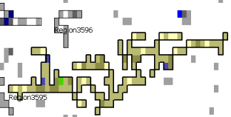 |
Left: Two example regions and their associated Image compactness values Region3596: IC = 20.8 Region3595: IC = 155.8 Note: An Image compactness of -1 indicates the region has no GPS value. |
Corrected_mean_amplitude
Ec = En · (A2D / A)· 10(dRvc/10) if A ![]() 0;
0;
Ec = 0 if A = 0
Corrected_MVBS [Corrected mean volume backscattering strength (Sv)]
Rc = 10 log(Ec) if Ec> 0;
Rc = -999 if Ec ![]() 0
0
Coefficient_of_variation [Coefficient of variation of the amplitude energy]
ECV = ESD . 100 / Ec if Ec![]() 0;
0;
ECV = 0 if Ec = 0
![]()
Horizontal_roughness_coefficient
Horizontal_roughness = Rh2 / En
where Rh2 = Σj [(Ej - Ej+1)2 / (nh - 1)]
summation is over all horizontal pairs of samples in the region
nh is the number of horizontal pairs of samples within the region
Notes:
-
- The special export value for an invalid calculation is -9.9e+37. An aborted calculation can occur when the sample count changes between pings.
- The algorithm excludes pairs that have thresholded values (-999) from the numerator and denominator. Effectively, the roughness is based on the above-threshold samples in the detected school.
Vertical_roughness_coefficient
Vertical_roughness = Rv 2 / En
where Rv2 = Σk [(Ek – Ek+1)2 / (nv - 1)]
summation is over all vertical pairs of samples in the region
nv is the number of vertical pairs of samples within the region
Notes:
-
- The special export value for an invalid calculation is -9.9e+37.
- From Echoview 5.2, to maintain consistency with the Horizontal_roughness, the Vertical_roughness algorithm excludes pairs that have thresholded values (-999) from the numerator and denominator. Previously, the algorithm excluded thresholded pairs from the numerator then counted them in the denominator. In that case, below-threshold samples would tend to increase the Vertical_roughness. In practice, a threshold is applied, then a school detection is run and the School Detection module analysis variables are exported. Under that regime, detected schools would contain few thresholded samples, and the effect on Vertical_roughness would be minimal.
3D approximations - available with School Detection module only
3D_school_volume (assuming cylindrical shape, 3D)
School volume:
V = Σj π . (Tj/2)2 . Lj
where:
j is the ping number
Tj is the thickness of the region at ping j
where:
Tj = Σi Ti
Ti is the size of sample interval i in ping j, such that:
Ti = 0 when Ti is associated with a sample:
- above an Exclude Above line
and/or
- below an Exclude Below line
and/or
- that is a no-data sample and Include the volume of no-data samples is not selected
Ti otherwise.
Lj is the distance from ping j to ping j+1 as determined using the Position source selected on the Position page of the Platform Properties dialog box (exception: for the last ping in the region only, it is the distance from ping j-1 to ping j).
Corrected school volume:
Vc = V . (Tc2 . Lc) / (T2 . L) if (T2 . L) ![]() 0;
0;
Vc = 0 otherwise.
Formulae for calculating other region variables using SHAPES algorithms - available for export with Essentials module and/or the School Detection module
Ping_M [Mean ping number]
Ping number of middle ping of bounding rectangle. See Ping_M algorithm.
Lat_M and Lon_M [Mean Latitude/ Longitude]
Latitude and longitude of middle ping (pm). See Lat_M and Lon_M.
Range_mean and Depth_mean [Mean School Range and Depth]
Mean of range or depth of all good data points in region. See Range_mean and Depth_mean.
See also About Transducer Geometry and About depth, range and altitude.
Mean distance from Bottom
This is not output, but can be calculated as the mean bottom depth/range (Exclude_below_line_depth_mean / Exclude_below_line_range_mean; if the exclude below line is the bottom) minus mean school depth/range (Depth/Range_mean) depending upon the choice or depth or range modes.
Time_M and Date_M [Mean time and date]
Date and time of middle ping (pm). See Time_M and Date_M.
VL_mid [Mean log marker]
Vessel log distance for middle ping (pm). See VL_mid.
Dist_mid
The GPS distance of the middle ping can also be calculated. See Dist_M.
Skewness
Skewness is a statistic that is used to measure the symmetry of the distribution for a set of data. See About skewness and Skewness algorithm.
Kurtosis
Kurtosis is a statistic that is used to measure the "flatness" or "peakedness" of a set of data. See About kurtosis and Kurtosis algorithm.
See also
Notes about school detection
School Detection module references
School detection while live viewing algorithm