Background Noise Removal

This operator estimates the background-noise level and subtracts it from the value of each sample. Background noise can manifest as TVG-noise striping on an echogram. The Background noise removal algorithm is based on concepts from De Robertis and Higginbottom (2007). The algorithm page also offers practical advice on background noise removal strategies.

On the Background Noise Removal page of the Variable Properties dialog box, you can specify four parameters to configure the averaging cell used to determine the noise estimate. You can also specify two values to put a limit on acceptable noise and SNR.

Notes:

• See also: The Data thresholding section on the Noise, background object and signal removal in Echoview page.
• See also: The Effect of No data samples on the Wideband Frequency Response graph page.
• TVG is not applied at ranges less than 1 meter from the transducer.

Echoview accepts operands of the following data type as input:

• Complex power dB
• Complex Sv
• Complex TS
• Multibeam Sv
• Multibeam TS
• Power dB
• Pulse compressed complex power dB
• Pulse compressed complex Sv
• Pulse compressed complex TS
• Sv
• TS

Settings

The Background Noise Removal Variable Properties dialog box pages include (common) Variable Properties pages and these operator pages:

Operands page

Background Noise Removal page

The following settings are used by the Background noise removal algorithm which is based on the concepts discussed by De Robertis and Higginbottom (2007). The algorithm page also offers practical advice on background noise removal strategies.

Note: If the calibration of the selected beam differs from that of beam 0 then the correct values should be supplied using an ECS file. Unintended values may otherwise result.

Averaging Cell

Settings that configure the averaging cell that is used to find the noise estimate of each ping.

Settings	Description
Horizontal extent (pings)	Specifies the horizontal size of the averaging cell (number of pings). The cell width defines an averaging ping interval that examines samples for the noise estimate for the middle ping of the interval. The default value is 20 pings. The value is cited in the Sensitivity to grid size discussion in De Robertis and Higginbottom (2007).
Vertical units	Specifies the units for the vertical axis of the averaging cell. Available units are Samples or Meters. Notes: Under Meters, a value for samples per meter is evaluated once (only), for the first group of calibrated pings and is applied to all pings in the echogram. In the case where the ping calibration changes within the data, the evaluated value may be inaccurate. Meters are used in De Robertis and Higginbottom (2007).
Vertical extent (samples) Vertical extent (meters)	Specifies the vertical size of the averaging cell. Notes: De Robertis and Higginbottom (2007) use a vertical cell size of 10 m for their data. The number of samples within the Vertical extent of the averaging cell can affect the statistics of the noise estimate. Too few samples may result in a poor noise estimate. Be aware that too few samples may result in a poor noise estimate.
Vertical overlap (%)	Specifies the percentage vertical overlap of the averaging cell down the samples of the averaging ping interval. Notes: The default overlap is zero. De Robertis and Higginbottom (2007) use non-overlapping averaging cells. Calculation time increases with an increase in Vertical overlap. The maximum overlap that can be entered is 99%. Specify an overlap when the calculated noise estimate is too high and erodes the wanted signal. Echogram results may change for dataflows that use Vertical overlap (%) due to a fix for this setting from Echoview 10.

Thresholds

Settings that specify the limits of acceptable noise and SNR for the operand data.

Settings	Description
Maximum noise (dB)	Specifies the maximum acceptable noise (dB) for the operand data. The algorithm uses this value when the calculated noise is greater than the Maximum Noise. The single beam default value is -125 dB. De Robertis and Higginbottom (2007) use this value for their data. Maximum Noise is equivalent to Noisemax used by De Robertis and Higginbottom (2007). "...Noisemax represents an upper limit for background noise expected under the operating conditions. Noisemax must be determined empirically and will depend on the echosounder, its installation, and the radiated noise of the vessel." Note: The Maximum noise (dB) threshold default value used for single beam is not appropriate for multibeam because multibeam data is often not constrained to the -70 .. 0 dB range common with single beam. A default of 999.0 dB is used for multibeam and it is advised to adjust this to a value suitable for the data.
Minimum SNR	Specifies the acceptable signal-to-noise ratio (dB) for samples in the operand data. The algorithm evaluates the noise-corrected-signal to calculated-noise ratio and tests to see it satisfies a minimum desired SNR. If the ratio is less than Minimum SNR then the signal is deemed not to be acceptably distinguishable from the noise. In this case, the corrected Sv is set to -999. The default value is 10 dB. Minimum SNR is equivalent to thresholdSNR used by De Robertis and Higginbottom (2007). "...SNR is a measure of the relative contribution of signal and noise and can be used objectively to identify data that contain sufficient signal to warrant further analysis, such as echo integration or multifrequency comparisons...The minimum thresholdSNR required to suppress the contribution from these pixels can be estimated by examining distributions of Powercal from areas dominated by noise and selecting a threshold above the mean value that will exclude contributions from it. This value will depend on the equipment used, the operational settings, and the extent to which data are averaged..."

Algorithm

The Background noise removal operator algorithm removes background noise for Sv, TS, power dB, multibeam Sv or multibeam TS variables. The algorithm estimates the noise for each ping and subtracts it.

You can specify six settings on the Background Noise removal page of the Variable Properties dialog box. Four settings specify the size and nature of the averaging cell used to determine the noise estimate. Two Threshold settings specify the Maximum Noise and Minimum SNR for the algorithm.

The algorithm is based on concepts discussed in "A post-processing technique to estimate the signal-to-noise ratio and remove echosounder background noise." by A. De Robertis and I. Higginbottom (2007).

• De Robertis and Higginbottom (2007) Abstract
• Background noise removal algorithm summary
  • Notes
  • Points of difference
  • TS, multibeam and complex data
• Practical advice
• Algorithm
  • Figure: Averaging cell
  • Figure: Averaging ping interval and averaging vertical intervals
  • Measured Sv and (noise) Corrected Sv
  • Estimate the noise
  • Remove the noise

De Robertis and Higginbottom (2007) Abstract

"A simple and effective post-processing technique to estimate echosounder background-noise levels and signal-to-noise ratios (SNRs) during active pinging is developed. Similar to other methods of noise estimation during active pinging, this method assumes that some portion of the sampled acoustic signal is dominated by background noise, with a negligible contribution from the backscattered transmit signal. If this assumption is met, the method will provide robust and accurate estimates of background noise equivalent to that measured by the receiver if the transmitter were disabled. It provides repeated noise estimates over short intervals of time without user intervention, which is beneficial in cases where background noise changes over time. In situations where background noise is dominant in a portion of the recorded signal, it is straightforward to make first-order corrections for the effects of noise and to estimate the SNR to evaluate the effects of background noise on acoustic measurements. Noise correction and signal-to-noise-based thresholds have the potential to improve inferences from acoustic measurements in lower signal-to-noise situations, such as when surveying from noisy vessels, using multifrequency techniques, surveying at longer ranges, and when working with weak acoustic targets such as invertebrates and fish lacking swim bladders."

Algorithm summary

The Background Noise Removal algorithm assumes that some portion of the sampled acoustic signal is dominated by background noise. It estimates the background noise value for each ping and subtracts it from the ping's samples. The algorithm analyzes the echogram by averaging the sample values, with TVG removed, within averaging cells around each ping. The averaging cells have a fixed horizontal extent in pings and a fixed vertical extent in samples. The noise estimate for a ping is the minimum of its cell averages. The estimate is thresholded against Maximum Noise and the result, with appropriate TVG added, is subtracted from each sample. If the result is less than the Minimum SNR it is set to -999.

The averaging cell is specified by four settings:

• Horizontal extent
• Vertical units
• Vertical extent
• Vertical Overlap

The Horizontal extent defines the width of the averaging cell, which is the averaging ping interval around the central ping. The interval moves across the echogram one ping at a time, so that ping to ping noise removal is smooth.

The Vertical extent defines the height of the averaging cell. Averaging cells vertically divide the samples in an averaging ping interval. A smaller height is more affected by spuriously low values. A larger height is more likely to contain traces of signal.

The Vertical overlap defines the amount that successive cells overlap vertically. The overlap helps to search out regions of pure noise between samples containing signal. The larger the overlap, the larger the number of cells processed, and hence the longer the processing time. If your data has few areas of pure background noise, the algorithm may have difficulty finding them, and the calculated value may exceed the maximum noise in some places. In that case you can specify a vertical overlap between cells. This increases processing time but makes the noise estimate search more thorough.

Notes:

• At the edges of the data, the sliding window stops sliding but does not shrink at the ends. The first pings i = [0, Horizontal extent/2] have the same noise estimate. The last pings i = [(Last - Horizontal extent/2), Last ping] have the same noise estimate. These pings cannot be at the center of a ping interval. Therefore the algorithm assigns these pings the noise estimate for the middle ping of the nearest valid ping interval k.
• The effectiveness of the Background noise removal operator relies on finding data that is dominated by background noise. An area that is more likely to include such data is the area below the acoustic bottom. This suggests that there is value in including below bottom samples in your data.
• See also: Data Thresholding section on Noise, background object and signal removal in Echoview.
• See also: Wideband considerations.

Points of difference

The implementation is slightly different to that used by De Robertis and Higginbottom (2007). The points of difference are:

• Averages are calculated around a ping, so that each ping has its own noise estimate. De Robertis and Higginbottom apply the same noise estimate to all the pings in the averaging time interval.
• Averaging cells can be overlapped vertically. De Robertis and Higginbottom use non-overlapping averaging cells.
• The last vertical interval can overlap the second-last vertical interval, when Vertical extent and Vertical Overlap(%) do not evenly divide the samples in a ping. The Figure: Intervals illustrates this for zero Vertical overlap and for a non-zero Vertical overlap.

TS, power, multibeam, complex, and pulse compressed complex data

The Background noise removal operator algorithms accommodate TS, Power, multibeam, complex and pulse compressed complex data. Note that De Robertis and Higginbottom (2007) do not examine TS/multibeam/complex noise estimation or removal.

• TS and Power operands are handled in a similar way to Sv operands.
• Aspects of TS noise estimation using split-beam TS data are discussed by Kieser et al (2005). Kieser et al observations provide a guide to TS noise estimation and TS noise removal.
• When applied to multibeam data, this operator takes the calibration settings from beam 0 of the operand. If calibration differs significantly across the beams then the correct values should be supplied using an ECS file. Unintended values may otherwise result.
• Complex and pulse compressed complex acoustic variables are largely handled in a manner similar to single frequency power, Sv or TS variables. When a new sample value is required, it is assumed that the complex phase for the sample is unchanged and the complex magnitude of the sample is calculated as for ComplexMagnitudeNew.

Practical advice

The background noise removal operator works very well on averaged data. Under averaged data, the mean background noise does not change but its variance decreases. De Robertis and Higginbottom (2007) argue and demonstrate this in their discussion directed to Figure 2 in their paper.

The minimum SNR threshold value required to suppress noise depends on the degree to which input data are averaged.

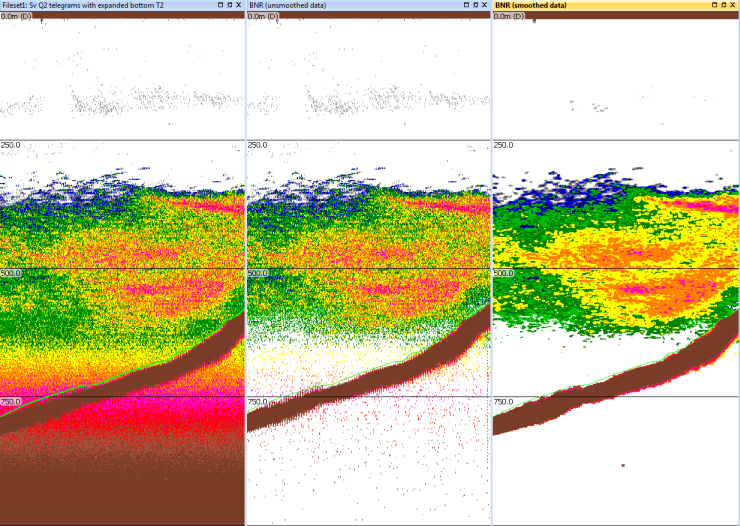
From left to right:

• Original data - 120 kHz echogram shows an aggregation of walleye pollock in the Bering Sea with TVG amplified background noise
• Unsmoothed data into Background noise removal operator, Minimum SNR = 1.00
• Smoothed data (via 5 x 5 convolution) into Background noise removal operator, Minimum SNR = 1.00

In this case for low Minimum SNR, it is clear that smoothing is preferable because it removes the ‘speckly’ noise that is visible above background in the smoothed data (i.e., the method computes the noise level relative to the mean noise level, and some samples will be substantially above if unsmoothed). The smoothed and unsmoothed data become more alike as the Minimum SNR is raised.

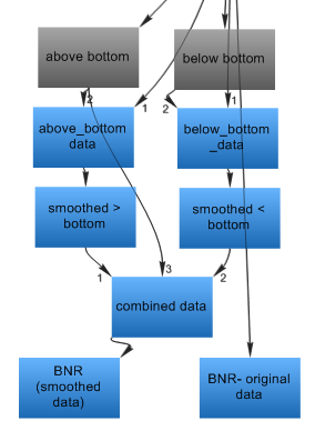
SNR criteria are best applied at a resolution larger than one pixel. A useful approach is to smooth/average above-bottom and below-bottom data separately. Then combine the results with a Select operator after averaging so that the bottom is not combined with near-bottom data above the SNR.

A dataflow to achieve this is:

Virtual variable name Operator Aim below bottom above bottom Line bitmap Create a bitmap of the area between two specified lines. above_bottom data below_bottom_data Mask Apply bitmap mask to data. smoothed > bottom smoothed < bottom 5 x 5 convolution Smooth the data. combined data Select Uses a bitmap to select values from two variables: above_bottom bitmap smoothed > bottom data smoothed < bottom data BNR (smoothed data) BNR - original data Background noise removal Apply Background noise removal algorithm with SNR criteria.

Algorithm

The algorithm is described for an Sv operand. When a TS operand is used, the following are substituted for Sv quantities: TS values, the equation for TS(Range, Power) and TS nominal TVG(Range).

When a Power operand is used, the following are substituted for Sv quantities: Power values.

Averaging cell

Averaging ping interval and averaging vertical intervals

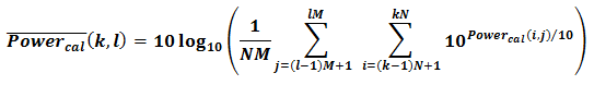
is used to estimate the noise in the interval.

Where:

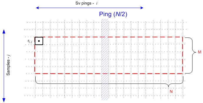
M	=	The height of the averaging cell. M is specified by Vertical extent (samples) or Vertical extent (meters) on the Background Noise Removal page of the Variable Properties dialog box. De Robertis and Higginbottom (2007) define their averaging cell in terms of M samples and N pings.
N	=	The width of the averaging cell. N is specified by Horizontal extent (pings) on the Background Noise Removal page of the Variable Properties dialog box. De Robertis and Higginbottom (2007) define their averaging cell in terms of M samples and N pings.
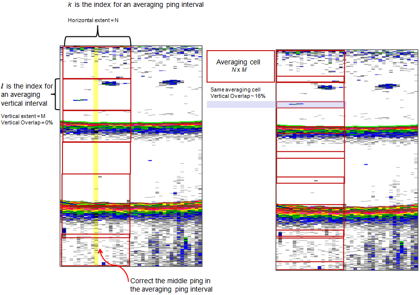
k, l	=	k is the index for an averaged ping interval. The noise estimate for an averaged ping interval's central ping is a result of the vertical consideration of samples within the ping interval. l is the index for the averaged vertical intervals. The vertical consideration of samples within an averaged ping interval is achieved by examining results from averaged vertical intervals. The number of averaged vertical intervals is determined by the averaging cell height M and the specified Vertical overlap. Both types of intervals are illustrated in the Figure: Intervals and further implementation detail is in Algorithm summary: Notes and Algorithm summary: Points of difference. De Robertis and Higginbottom (2007) define k as the index for the averaged time interval. They define l as the index for the averaged vertical intervals. Their averaging cells do not overlap (vertically) and their noise estimate for the averaged time interval was applied to all pings in the interval.
Vertical overlap	=	The percentage overlap of the vertical averaging cells. This is illustrated in the Figure: Intervals. Further detail about Vertical overlap is in the Algorithm summary. This is Vertical overlap (%) on the Background Noise Removal page of the Variable Properties dialog box.
ri, j	=	The uncorrected range (m) for the center of sample j in ping i.
rtvg(i, j)	=	The TVG corrected range (m) for the center of sample j in ping i. The TVG correction to the range is a function of the AbsorptionCoefficient, SoundSpeed, and PulseDuration. These quantities and the TVG range correction algorithm are taken from the ping's calibration settings. Note: The corrected range can also be written as R(i, j).

• Measured Sv and (noise) Corrected Sv
• Estimate the noise
• Remove the noise

Measured Sv and (noise) Corrected Sv

The Background Noise Removal algorithm assumes that some portion of the sampled acoustic signal is dominated by background noise, with a negligible contribution from the backscattered transmit signal. This is expressed in the equation for Sv, meas.

By examining Sv, meas, an Sv, noise value can be estimated and a background-noise-corrected Sv can be calculated.

Note: For a TS operand, TS values and TS equations are used. For a Power operand, Power values are used.

Sv, meas(i, j)	=	Measured mean volume-backscatter strength (dB re 1m-1) of sample j in ping i. where: Sv, signal(i, j) is the contribution from the backscattered transmit pulse (dB re m-1) of sample j in ping i. Sv, noise(i, j) is the contribution from the noise (dB re m-1) of sample j in ping i. De Robertis and Higginbottom (2007) "The primary assumptions of the method are that background noise is independent of elapsed time during one transmit-and-receive cycle, and that at some point in the measured cycle, the measurement is dominated by contributions from background noise (i.e., Sv,noise >> Sv,signal). This assumption means that noise “spikes” such as short-duration interference from the transmit signal of other echosounders are not present, or have been excluded from the data. If these assumptions are met, a portion of the return observed from an active ping (i.e., transmitter enabled) will give similar readings to those of an echosounder in passive mode, which is a measurement of background noise (Figure 1). If this assumption is violated, this and other methods (e.g. Kloser, 1996; Watkins and Brierley, 1996; Higginbottom and Pauly, 1997; Korneliussen, 2000) based on active pinging will overestimate noise because the portion of the measurement used to estimate noise levels will include appreciable backscattered signal as well as background noise."
Sv, corr(i, j)	=	Corrected Sv (dB re 1m-1) of sample j in ping i.

Estimate the noise

The algorithm averages the samples within each cell of an averaging ping interval. The minimum result is the noise estimate for the ping at the center of the ping interval.

Note: For a TS operand, TS values and TS equations are used.

1. Calculate the average Powercal for samples within each vertical interval l of a ping interval k.

=

Resample Powercal(i, j) by averaging the samples in the vertical intervals of an averaging ping interval. where: Powercal is nominally the logarithmic measure of received power (adjusted for the echosounder-specific calibration coefficients) used in echo integration, i.e., Sv,meas with the TVG removed. l is the index for the vertical intervals in an averaging ping interval k. The number of vertical intervals is specified by Vertical extent and Vertical Overlap(%) and the arrangement of the intervals over the total number of samples in a ping. Note: When calculating , any cell that contains fewer than one ping's valid samples is ignored. For example, given a cell height of 5 samples and width of 10 pings, any cell with fewer than 5 valid samples (hence more than 45 no_data samples) is ignored.

2. The noise estimate for the middle ping in interval k, is the minimum value of the vertical intervals l.

3. Test this estimate against the acceptable Maximum Noise value.

Maximum Noise

=

The maximum acceptable value for the calculated noise (dB) for the operand data. If the calculated noise exceeds Maximum Noise, Maximum Noise is used instead. This is Maximum Noise on the Background Noise Removal page of the Variable Properties dialog box. Maximum Noise is equivalent to Noisemax used by De Robertis and Higginbottom (2007).

If Noise(k) > Maximum Noise then set Noise(k) = Maximum Noise.

Remove the noise

Note, for a TS operand, TS values and TS equations are used. For a Power operand, Power values are used.

1. For the middle ping of the averaging ping interval k, remove the noise from the Sv values in the ping.

Sv, corr(i, j)

=

Noise-corrected mean volume-backscatter strength (dB re 1m-1) of sample j in ping i. where: Sv, meas(i, j) = Measured mean volume-backscatter strength (dB re 1m-1) of sample j in ping i. Noise (i) is the noise estimate for ping interval k and is equal to Noise(k).

2. Test this against the acceptable Minimum SNR value.

Minimum SNR

=

The acceptable signal-to-noise ratio (dB) for samples in the operand data. If the signal-to-noise ratio of a noise-corrected sample is less than or equal to Minimum SNR, the Sv is set to -999. This is Minimum SNR on the Background Noise Removal page of the Variable Properties dialog box. Minimum SNR is equivalent to thresholdSNR used by De Robertis and Higginbottom (2007).

The signal-to-noise ratio can be expressed as SNR(i, j) = Sv, corr(i, j) - Sv, noise(i, j)

If SNR(i, j) is less than or equal to Minimum SNR then set Sv, corr(i, j)= -999.

3. The first pings i = [0, Horizontal extent/2] have the same noise estimate. The last pings i = [(Last - Horizontal extent/2), Last ping] have the same noise estimate. See also Algorithm summary: Notes.
4. When a ping is in the set of pings [0...N/2], use the noise estimate of ping N/2 of the first valid ping interval at noise-removal step 1.
5. When a ping is in the set of pings [(Last ping-N/2)...Last ping], use the noise estimate of ping (Last ping - N/2) of the last valid ping interval at noise-removal step 1.

See also

About virtual variables
Operator licensing in Echoview
Background noise in Echoview
Background noise calculation on the Analysis page
Impulse noise removal operator
Transient noise sample removal operator
Using a SoundSpeedProfile: Notes