Match geometry algorithm
The Match geometry operator resamples Operand 1 to match the ping geometry of Operand 2. This virtual variable is useful for modifying the ping geometry of an operator in preparation for dB differencing and when you need to return resampled data to its original ping geometry.
Ping geometry is read from the data file and includes:
- Ping start range
- Ping stop range
- Number of samples per ping
The resampling is a weighted mean calculation.
Notes:
- The Match geometry operator can upsample or downsample. Ping times for Operand 1 and 2 must match. See also: Match ping times operator.
- Echoview offers various Resample operators that provide additional resampling options.
- For data with units in dB, the weighted mean is calculated in the linear domain.
Figure 1: Illustration for Match geometry resampling. Representative pings, samples and sample start range and sample stop range are displayed. In this example, the values at the sampling frequency of Operand 1 are downsampled (reduced resolution, reduced sampling rate) via weighted mean to the sampling frequency of Operand 2. The value of sample1 in the Match Geometry Output ping (right) is the weighted mean of Operand 1 samples: x1, x2, and partial x3 in the range ry0 to ry1 as shown. The sampling frequency for any ping can be viewed in the Details pane or on the Calibration page of the Variable Properties dialog box.
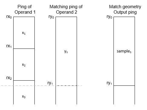
Illustration definitions (Figure 1)
Ping geometry of pings in Operand 1
xN is the Nth sample of a ping in Operand 1. Sample xN start range in meters (rxN-1) and sample stop range in meters (rxN) are derived from the ping geometry of Operand 1.
v(xN) is the value of the Nth sample of a ping in Operand 1.
Ping geometry of pings in Operand 2
yM is the Mth sample of a matching ping in Operand 2. Sample yM start range in meters (ryM-1) and sample stop range in meters (ryM) are derived from the ping geometry of Operand 2.
Ping geometry of pings in Match geometry pings
sampleM is the Mth sample of the Match geometry ping. The ping geometry is that of Operand 2.
v(sampleM) is the value of the Mth sample of the Match geometry ping.
Calculations for the value of an output sample consider the weighted mean contribution of samples in Operand 1 to the output sample with the ping geometry of Operand 2.
- Where an Operand 1 sample is completely within the boundaries of the output sample, the weighting for the Operand 1 sample is w = 1.
- Where an Operand 1 sample partially overlaps the output sample, the weighting for the Operand 1 sample is w.
- w is calculated as the part of the Operand 1 sample that overlaps the output sample divided by the Operand 1 sample thickness.
Example calculation for the first sample of the output ping in Figure 1
| Operand 1 sample index xi |
Operand 1 sample weight wi |
Match geometry virtual variable |
| x1 with v(x1) | w1 =1 |  |
| x2 with V(x2) | w2 =1 | |
| x3 with v(x3) |  |
Figure 2: Representative pings, samples, and sample start and stop ranges are displayed. In this example, values at the sampling frequency of Operand 1 are upsampled (increased resolution, increased sampling rate) using weighted-mean resampling to match the sampling frequency of Operand 2. For data in dB, the weighted-mean calculation is performed in the linear domain before the result is converted back to dB. When data are upsampled, each Operand 1 sample contributes proportionally to multiple smaller-range output samples. In this figure, the –45.6 dB output sample is calculated from 2/3 of the –50 dB Operand 1 sample and 1/3 of the –42 dB sample, reflecting their geometric overlap. This example also illustrates a potential artifact near the seafloor–water column interface: strong bottom returns may be redistributed to shallower ranges, creating the appearance of “bottom leakage”. If the bottom boundary for Operand 1 is defined between –42 dB and –50 dB, the upsampled data may include redistributed bottom energy above the true boundary. The sampling frequency for a ping can be calculated from information reported in the Details pane, such as Data range, Data points, and Sound speed (for example, Data range = 186.06 m, Data points = 12475, and Sound speed = 1491.49 m s–1, which results in a sampling frequency of 50.0 kHz).

Illustration definitions (Figure 2)
Ping of Operand 1 (left column)
Shows three representative sample values from Operand 1, colored according to the EK500 color scale (–50 dB, –42 dB, –38 dB). The height of each colored block reflects the sample height in Operand 1.
The dashed lines indicate the boundaries where samples contribute to the weighted mean used in the upsampling process.
Operand 2 geometry (middle column)
Shows how Operand 2 has a finer sampling frequency (smaller sample heights). These smaller sample intervals define the target geometry for the Match geometry operator.
No sample values are shown because the purpose of this column is solely to illustrate sample heights as defined by the ping geometry of Operand 2.
Match geometry Output ping (right column)
Shows the resulting upsampled data, with sample values calculated by combining portions of the Operand 1 samples according to geometric overlap.
For example, the –45.6 dB sample is composed of 2/3 of the –50 dB sample and 1/3 of the –42 dB sample, as indicated by the dashed lines.
The lower sample fades out to suggest continuation (only a subset of samples is shown).
For data in dB, the weighted-mean calculation is performed in the linear domain (power units) before being converted back to logarithmic form for display in dB. This ensures proportional weighting accurately represents the contribution of each Operand 1 sample to the upsampled output.
Dashed construction lines
Dashed lines illustrate geometric boundaries and proportional contributions between Operand 1 samples and the output samples.
These lines visually clarify how sample overlap determines weighting when calculating each upsampled sample value.