GLCM Texture Feature
This operator produces a virtual variable which represents a GLCM texture image of a single beam echogram.
It accepts a single operand of one of the following data types:
- Linear
- Power dB
- Sv
- TS
- Unspecified dB
Settings
The GLCM Texture Feature Variable Properties dialog box pages include (common) Variable Properties pages and these operator pages:
Operands page
GLCM Texture page
This page allows you to select GLCM, gray level and texture feature settings.
|
Setting |
Description |
||||||||
|
Feature |
Select a GLCM texture feature from the list: |
||||||||
|
Window size |
Specifies the window size for the GLCM texture feature. The window size defines the area of samples used for GCLM tabulations and texture calculations.
|
||||||||
|
Quantization |
Specifies parameters so that sample intensity can be assigned to discrete gray levels for the calculation of the GCLM. Each gray level represents a range of sample intensity values.
Notes:
|
||||||||
|
Spatial Relationship |
Defines the spatial relationship between the reference sample and the neighbor sample used in tabulations for the GLCM. For example:
|
About the GLCM and textures
The Gray Level Co-occurrence Matrix1 (GLCM) and associated texture feature calculations are image analysis techniques. Given an image composed of pixels each with an intensity (a specific gray level), the GLCM is a tabulation of how often different combinations of gray levels co-occur in an image or image section. Texture feature calculations use the contents of the GLCM to give a measure of the variation in intensity (a.k.a. image texture) at the pixel of interest.
Echoview offers a GLCM Texture Feature operator that produces a virtual variable which represents a specified texture calculation on a single beam echogram.
Algorithm
The virtual variable is created in the following way (using the settings on the GLCM Texture page of the Variable properties dialog box identified in bold):
- Quantize the image data. Each sample on the echogram is treated as a single image pixel and the value of the sample is the intensity of that pixel. These intensities are then further quantized into a specified number of discrete gray levels as specified under Quantization.
- Create the GLCM. It will be a square matrix N × N in size where N is the Number of levels specified under Quantization. The matrix is created as follows:
- Let s be the sample under consideration for the calculation.
- Let W be the set of samples surrounding sample s which fall within a window centered upon sample s of the size specified under Window Size.
- Considering only the samples in the set W, define each element i,j of the GLCM as the number of times two samples of intensities i and j occur in specified Spatial relationship (where i and j are intensities between 0 and Number of levels-1).
The sum of all the elements i, j of the GLCM will be the total number of times the specified spatial relationship occurs in W. - Make the GLCM symmetric:
- Make a transposed copy of the GLCM
- Add this copy to the GLCM itself
This produces a symmetric matrix in which the relationship i to j is indistinguishable for the relationship j to i (for any two intensities i and j). As a consequence the sum of all the elements i, j of the GLCM will now be twice the total number of times the specified spatial relationship occurs in W (once where the sample with intensity i is the reference sample and once where the sample with intensity j is the reference sample), and for any given i, the sum of all the elements i, j with the given i will be the total number of times a sample of intensity i appears in the specified spatial relationship with another sample.
- Normalize the GLCM:
- Divide each element by the sum of all elements
The elements of the GLCM may now be considered probabilities of finding the relationship i, j (or j, i) in W.
- Divide each element by the sum of all elements
- Calculate the selected Feature. This calculation uses only the values in the GLCM. See:
- The sample s in the resulting virtual variable is replaced by the value of this calculated feature.
Texture equations
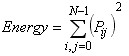
Energy feature
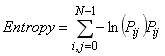
Entropy feature
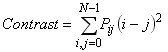
Contrast feature
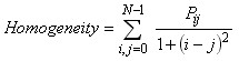
Homogeneity feature
Correlation feature
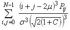
Shade feature
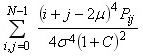
Prominence feature
Where:
Pij = Element i,j of the normalized symmetrical GLCM N = Number of gray levels in the image as specified by Number of levels in under Quantization on the GLCM texture page of the Variable Properties dialog box. = the GLCM mean (being an estimate of the intensity of all pixels in the relationships that contributed to the GLCM), calculated as:
Note: This also approximates, but is not identical to, the mean of all the pixels in the data window W (as defined by the GLCM algorithm), and it is dependent upon the choice of spatial relationship in that algorithm.
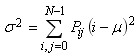
= the variance of the intensities of all reference pixels in the relationships that contributed to the GLCM, calculated as:
Note: This may approximate, but is not identical to, the variance of the intensities of all the pixels in the data window W (as defined by the GLCM algorithm), and it is dependent upon the choice of spatial relationship in that algorithm.
= = The Correlation feature sgn(x) = Sign of a real number
x = -1 for x < 0
x = 0 for x = 0
x = 1 for x > 0=
See also
About virtual variables
Operator licensing in Echoview
1. Newcomers to this topic are advised to read the GLCM Tutorial at https://prism.ucalgary.ca/handle/1880/51900 and pursue any further reading if necessary.