XxYxZ Convolution
This operator applies an XxYxZ convolution algorithm to the echogram.
Operand 1 |
|
You define the convolution algorithm and size of the convolution window on the XxYxZ Convolution page of the Variable Properties dialog box.
Notes:
- Under live viewing, the Live Export based on a convolution variable may be limited.
- The XxYxZ convolution operator assumes that the operand ping geometry does not change from ping to ping.
Settings
The XxYxZ Convolution Variable Properties dialog box pages include (common) Variable Properties pages and these operator pages:
Operands page
XxYxZ Convolution page
Specifies the convolution algorithm and the size of the convolution kernel window.
|
Setting |
Description |
|
Algorithm |
Select a convolution algorithm to use. |
|
Rows (samples) |
Specifies the row size of the convolution window. The row value is restricted to an odd number, between 1 and 999, and spans the multibeam sample space. |
Columns (beams) |
Specifies the column size of the convolution window. The column value is restricted to an odd number, between 1 and 999, and spans the multibeam beam space. |
|
Layers (pings) |
Specifies the z size (ping extent) of the convolution window. The column value is restricted to an odd number, between 1 and 999, and spans the multibeam ping space. |
|
Input samples per calculation |
Displays the number of input samples for each calculation. This number is based on the specified Row, Column and Layers settings. Although you can set Row, Column and Layers to any odd number between 1 and 999, it has been found that this operator's performance decreases as the product of these settings increases. A warning is displayed when the value for the Input samples per calculation is greater than 1000. |
Algorithm
Available XxYxZ Convolution kernel algorithms. For details on how kernel convolutions are applied and how new sample values are calculated in Echoview see Convolution algorithms: Sliding window and kernel.
Top hat algorithm
The cell kernel values in the XxYxZ convolution kernel are set to 1.
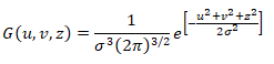
Gaussian blur algorithm
The Gaussian blur algorithm is an image-blurring filter that uses a normal distribution for calculating data values for the XxYxZ sliding window. The standard deviation σ is used to classify the "strength" of the blurring. The kernel cell values in the XxYxZ convolution kernel are calculated using the equation for a Gaussian distribution in three dimensions as follows:
Where:
u is the kernel row index (relative to the center [0,0,0]) of the specified sliding window.
v
is the kernel column index (relative to the center [0,0,0]) of the specified sliding window.
z
is the kernel z-plane index (relative to the center [0,0,0]) of the specified sliding window.
σ
is the standard deviation of the Gaussian distribution.
0.6 = weak
1.0 = moderate
2.0 = strong
More information on the Gaussian blur algorithm can be found in the Wikipedia topic Gaussian blur.