Convolution algorithms

Convolution operator calculations are applied in the linear domain.

Echoview's convolution operators fall into the following categories:

Convolution filter operators

Dilation filter nxn

Median filter nxn

Erosion filter nxn

Beam dilation filter 3x3

Beam median filter 3x3

Beam erosion filter 3x3

Beam opening filter 3x3

Beam closing filter 3x3

XxY statistic

XxYxZ statistic

Convolution kernel operators

nxn convolution

XxY convolution
XxYxZ convolution

Blur

Sharpen

Beam convolution 3x3

The algorithms and sample boundary issues are described below.

• Convolution filter operators
• Convolution kernel operators
• Edges
• Range changes

Please see Convolution operators illustrated for a graphic comparison of these operators.

Convolution filter operators

These operators apply a sliding window of either 3x3, 5x5 or 7x7 or XxY data points to the echogram. This window is centered in turn on each data point in the echogram and defines 9, 25, 49 or XxY values including the data point at the center and its neighbors (data points near the edges are a special case).

The value at the center of this window is replaced by a value specified by the convolution filter operator.

Type of operator	Value
Dilation	the maximum of the values within the window
Median	the median of the values within the window
Erosion	the minimum of the values within the window
XxY statistic	the statistic of values within the window on single beam data
XxYxZ statistic	the statistic of values within the window on multibeam data
Beam closing	applies a dilation to the entire echogram followed by an erosion
Beam opening	applies an erosion to the entire echogram followed by a dilation

Notes:

• Under live viewing, the Live Export based on a convolution variable may be limited.
• Under single beam convolution filter operators (Dilation, Median, Erosion and XxY statistic) and XxYxZ statistic, the algorithm checks adjacent pings in the convolution window. Pings with matching start ranges and matching sample thickness are evaluated. When an adjacent ping fails the check, its samples are left out of calculations.

Convolution kernel operators

• Sliding window and kernel
• Kernel sum is non-zero
• Kernel sum is zero
• Example convolution operators

Sliding window and kernel

These operators also apply a sliding window of either 3x3, 5x5, 7x7 data or XxY points to the echogram. This window is centered in turn on each data point in the echogram and defines 9, 25, 49, XxY or XxYxZ values including the data point at the center and its neighbors (data points near the edges are a special case).

Unlike the Convolution filter operators above they work with a kernel. This is an array of values, one value for each data point within the window - the kernel is the same size as the window.

For example a 3x3 convolution kernel may resemble:

0	0	0
0	1	0
0	0	0

The convolution is applied, by replacing the value of the data point at the center of the sliding window by a new value which is calculated by the convolution operator.

The new value is calculated differently depending on whether the sum of all the kernel cells is zero or non-zero. If the sum of all kernel cells:

• is non-zero (the more usual case), then the kernel is normalized (each kernel cell is divided by the sum of all kernel cells) before it is applied.

• is zero then the kernel is applied as-is; i.e. without normalization.

Notes:

• Under live viewing, the Live Export based on a convolution variable may be limited.
• Under single beam convolution filter operators (XxY Convolution and nxn Convolution), the algorithm checks adjacent pings in the convolution window. Pings with matching start ranges and matching sample thickness are evaluated. When an adjacent ping fails the check, its samples are left out of calculations.
• An XxYxZ convolution kernel may output unexpected results when sample and beam geometry change from ping to ping.
• The XxY and XxYxZ convolution can use a Top hat or a variation of a Gaussian blur kernel.

Kernel sum is non-zero

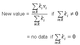
Where sum of all kernel cells is non-zero, the new value is calculated as follows:

Where:

R	is the region of convolution, i.e. the 3x3, 5x5, or 7x7 sliding window. The following cells will be excluded from the region of convolution: cells that contain a data point with a "no data" value cells that do not contain a data point, i.e. cells that fall outside boundary of the variable (see the Edges section for more information) cells that are on the "other side" of a range change in the variable (see the Range changes section for more information). Note: If cells are excluded from the region of convolution, the kernel is re-normalized before the new value is calculated. If it is not possible to normalize the kernel (because the sum of the data values in the remaining cells is zero) the new value of the data point is set to "no data".
i	is the number of a kernel cell (being 1 to 9, 1 to 25 or 1 to 49 respectively)
n	is the number of kernel cells (being 9, 25 or 49 respectively)
ki	is the value of the kernel cell i
vi	is the value in the sliding window cell i (being the value of a data point in the source variable).

Note:   Although "no data" points are not included in the calculation of new values for surrounding data points, they will be processed as per other kernel cells by convolution operators and may receive a new value from the convolution process. This may "patch up" holes in the data, i.e. calculate values for data points that were previously assigned a "no data" value (e.g. the data points may have been assigned a "no data" value to remove a data spike)

Kernel sum is zero

Where sum of all kernel cells is zero, the new value is calculated as follows:

Note: If any cells are excluded from the region of convolution (R), the new value will be "no data". This will result in eroded boundaries and "no data" areas being enlarged on the resulting virtual echogram (in comparison with when the source echogram).

Example convolution operators

The Blur and Sharpen operators are two specific cases of the general 3x3 convolution operator.

The convolution kernel used in the Blur operator is:

1	2	1
2	1	2
1	2	1

The convolution kernel used in the Sharpen operator is:

-1	-1	-1
-1	9	-1
-1	-1	-1

Edges

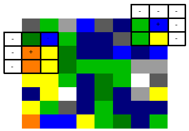
In the diagram below the cells marked '-' do not contain a data point (i.e. the sliding window is at the edge of the echogram). These cells will be excluded from the convolution region.

Range changes

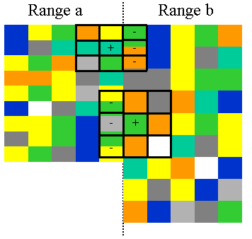
If the ping range changes in an echogram, neighboring pings are unlikely to line up in a precise grid. When this occurs, the cells in the sliding window that are not on the same side of the range change as the center cell are excluded from the convolution region. In the diagram below, cells that will be excluded from the two convolution regions are marked with "-".

You can ensure this does not occur by:

1. Creating a virtual variable that resamples the original operand using settings that will ensure that all pings will line up.

2. Changing the operand for the convolution virtual variable from the original variable to the resampled virtual variable.

Note: To check for range changes in the echogram, on the Echogram Display page of the Variable Properties dialog box, increase the value in the Lower display limit (m) box, until you can see the full range of each ping.

See also

Convolution operators illustrated
Operators
About virtual variables
References