Near-field depth
The near-field depth corresponds to the vicinity of the transducer's aperture where undesirable wave propagation effects reign in the transmitted ping. The signal from echoes within the near-field is generally unusable as the response is highly nonlinear in this zone.
In hydroacoustics, the near-field range is typically much less than 102 cm, but can theoretically extend to a few meters for low frequency systems with small beam angles.
Wave propagation in the near-field and far-field
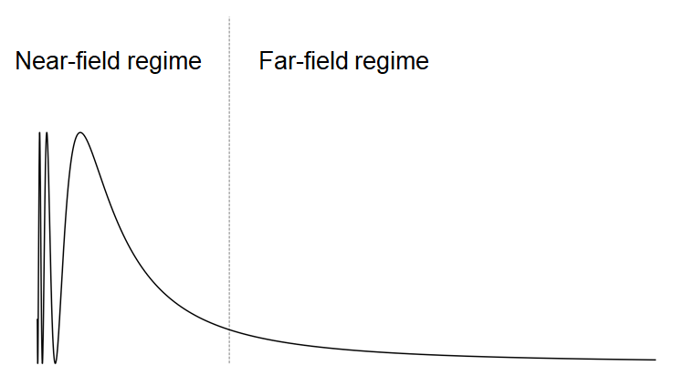
Each transmitted ping comprises many wavelets originating from piezoelectric elements in the transducer. As the individual wavefronts propagate, they expand in spherical shells. Within the near-field range of the transducer's beam, neighboring wavelets superimpose in complicated ways, resulting in constructive and destructive interference. The large fluctuations in the resulting wavefront require complex models to extract any signals that the echoes of the ping carry.
As the wavelets continue to expand beyond the near-field, the curved spherical arcs 'flatten' in the beam. This is the far-field where the wavefronts superimpose to form a uniform plane instead, and the amplitude of the resultant wavefront attenuates gradually with distance. It is more feasible to extract signals in the ping's echo from here.
The boundary between the near- and far-fields is not distinct. The transition between them varies with many factors, including the observation setup and the medium.
The Near-field depth estimation operator
The Near-field depth estimation operator infers the near-field range Rnf (cm) from the transducer frequency, 3dB beam angle and sound speed (refer to the Near-field range equation below). It also corrects for the transducer geometry (see below) and heave.
It outputs a depth line at 2×Rnf. You can adjust the constant factor using the Multiply near-field range by setting on the Line Properties dialog box.
Use this depth as a guide for where data is suitable for calibration and post-processing, for example with an exclusion line.
Other virtual or editable lines including reference lines for line-relative regions can accept the Near-field depth estimation line as an operand.
Near-field depth and transducer geometry
Echoview recomputes the near-field depth when the transducer geometry changes.
Figure 1 describes how the near-field depth varies with transducer geometry for an elevation angle of 0° (left) and between 0° and 180° (middle and right).
The pink hemispheres represent the near-field of the transducer. The pink isosceles triangles represent the beam and beam axis. In these examples, the azimuth and beam rotation are 0°.
When the elevation is not 0°, the transducer beam introduces a 'live' zone and amplifies the 'dead' zone. This can affect Sv and single target analysis.
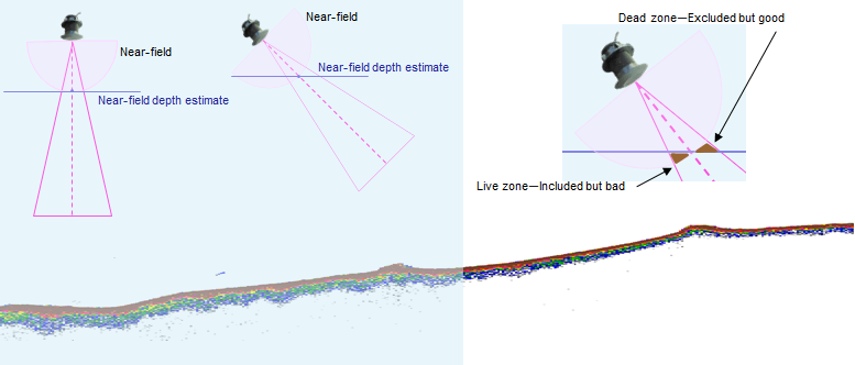
Figure 1. Near-field based range, near-field based depth line and zones that may affect analysis.
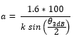
Near-field range equation
The near-field range Rnf (cm) is given by
![]()
from http://www2.dnr.cornell.edu/acoustics/Examples/NearfieldDistance/NearfieldDistance.html
Where: |
|
| a | Active radius (cm) of the transducer.
|

See also
About lines
About depth, range and altitude
Calibrating an echosounder
About analysis
About TVG: Nominal TVG