Calibrating an echosounder
This topic explains how to use the Calibration Assistant dialog box to output calibration offsets when working with calibration sphere data. Calibration Assistant input data are saved to the EV file, and one set of input data can be stored for each single target variable on the dataflow. This means it is possible to make a copy of a single target variable and store a different set of Calibration Assistant data against each instance of a single targets variable.
This page contains the following sections:
- Overview
- Calibration analysis features
- Using calibration sphere data
- Algorithms
- Two Way Beam Angle Correction
- Target envelope and Integrate samples using a nominated pulse length
- TS & Sv Offsets / Gain & Sa Correction
- Angle Offsets and 3dB beam angles
- Calibration sphere modeling and references
- NOAA FISHERIES Standard Sphere Target Strength Calculator
Notes:
- The techniques described in this topic are drawn from ICES CRR 326 Calibration of acoustic instruments (2015).
- For general information about calibration in Echoview, see About calibrated data.
- Example echograms for calibration sphere data can be seen here.
- Consult your manufacturer's guide for beam geometry calibration settings for your echosounder.
- See also the calibration in the context of the data processing workflow.
Overview
It is advised that you calibrate your echosounder before a survey. Echoview enables the entry of calibration values both in pre- and post-processing to achieve calibrated data values (e.g., TS, Sv values) from power data.
For echosounders that log raw power only (i.e., Echoview derives TS and/or Sv values from the power data), you may enter calibration settings in post-processing. For echosounders that log TS and/or Sv values you will need to calibrate your echosounder before the survey and may enter additional calibration settings during post-processing.
During calibration with a standard calibration sphere, calibration values in Echoview may be adjusted via an ECS file. The adjustments ensure that data values derived from power data are equal to the expected theoretical data values of the calibration sphere. The echosounder instrument system may also require the input of instrument and environmental calibration values for similar reasons.
In post-processing Echoview allows you to change instrument and environment calibration values through an ECS file. Some or all of the calibration settings determined when an echosounder is calibrated may be recorded in the data files Echoview reads. Values may not be reliably available in data files and there is also the possibility that values are not consistent for all files within a fileset. When required calibration values are absent from data files, Echoview uses default calibration values. As Echoview only permits one value per setting per variable for the whole fileset, it is up to you to determine which value to use if there is more than one value present in the data files within the fileset.
The information on this page is generally applicable calibrating both single beam and wideband data.
Important!
It is very important to ensure that you check your calibration values and verify they are correct. Note that default calibration values may be unsuitable for your data. To understand how calibrated data fits into Echoview's workflow, view the calibrated data workflow diagram.
Calibration analysis features
Echoview offers the Calibration Assistant dialog box to evaluate calibration sphere data and calculate:
- CalibrationOffsetTS or TransducerGain
- CalibrationOffsetSv or SaCorrectionFactor
- MinorAxisAngleOffset, MajorAxisAngleOffset (degrees)
- MinorAxis3dBBeamAngle, MajorAxis3dBBeamAngle (degrees)
- TwoWayBeamAngle corrected for SoundSpeed (dB re 1 sr)
- RMS error (dB)
Notes:
- The Essentials module is necessary to calculate calibration corrections using the Calibration assistant.
- Angular position data is used to calibrate beam shape.
- The Calibration Assistant Target Summary tab offers onscreen graphs and statistics. You can also save a report.
Other Echoview features that support the Calibration Assistant dialog box include:
- Echoview single target detection operators
- Live viewing
- Single target graphs - 2D projections and minor-axis and major-axis beam compensation graphs.
- Target samples bitmap operator and its Select sample using list.
- Use of the Cell Statistic operator to visualize aspects of the TS calibration calculation.
- Wideband frequency response graph configured with uncompensated TS or compensated TS for calibration sphere data.
- Export wideband frequency response TS data for a region on a single targets echogram.
- Echoview support for single target detection data added to a fileset. See Instrument file formats.
- ECS files to modify calibration values.
- COM EvVariableAcoustic.ExportSingleTargetCalibrationResults exports a text file with results from the Calibration Assistant Target Summary and new ECS values.
What benefits does Echoview provide?
Echoview can help you in the calibration process as follows:
|
Benefit |
Explanation |
|
Reduced time and cost associated with calibration |
You can collect calibration data in environmental conditions where it would not normally be possible, e.g., in rougher than optimal seas. The data you collect will contain both on-axis and off-axis single target detections, but you can filter out the off-axis targets and use only on-axis single targets for calibration. If you use Echoview in conjunction with one of Echoview Software's Echolog live viewing applications, you can monitor the collection of data in real time and collect only as much data as necessary to ensure statistically valid calibration, i.e., when you have enough on-axis single targets you can stop collecting calibration data, complete the calibration process, and begin your survey. |
|
Increased accuracy of calibration |
You can filter out off-axis single targets (these may be detected even in light seas) to ensure calibration is performed using only on-axis data. |
|
Appropriateness of calibration algorithms |
Echoview may use different algorithms to those used in your echosounder, e.g., for single target detection. You should calibrate using the same algorithms that you use to process your data. |
Check calibration in Echoview |
If you collect calibration data as part of your survey you can check the accuracy of user calibration settings during post-processing and adjust them as required to more accurately calibrate your data. Different variables can then be calibrated based on the core calibration data set. |
|
Calibration sensitivity analysis |
Calibration sensitivity analysis is facilitated by:
|
Using calibration sphere data to calculate calibration values
Calibration sphere echosounder narrowband or wideband data can be used to calculate Sv, TS, angle offset and beam width constants. The use of calibration constants means that calibrated data can be used for quantitative analysis.
TS and Sv calibration constants are values used in the equations that calculate TS values from power data or Sv values from power data. TS and Sv calibration constants match recorded on-axis single target calibration sphere data to expected theoretical calibration sphere values. The names of the TS and Sv calibration constants and their use in equations differs between echosounders but these constants' purpose is always the same (i.e., convert power data to TS or Sv data).
For TS or Sv variables derived from recorded power signals, Echoview assigns a nominal (default) associated calibration constant. This allows you to display an echogram for such variables immediately but the variable contains uncalibrated values as a result, which may be incorrect. Before you can draw any quantitative conclusion from your data you must enter the correct calibration constant. If you calibrated your echosounder before the survey you should replace the nominal value with a calibrated value. If you did not calibrate your echosounder prior to collecting survey data, or do not know these values, you can calibrate constants using the procedure described below.
Calibration sphere split-beam angular position data is required for the calculation of calibration constants for angle offsets and 3dB beam angles under suitable beam compensation models.
Notes:
- Power to Sv and TS equations differ by echosounder, see the relevant page in the Reference> Algorithms > Echosounders table of contents in this help file or contact Echoview support for more information.
- Calibration Assistant output values are unique to a single target variable. Use the Copy operator to duplicate a single target variable so that you can vary the inputs to the Calibration Assistant.
- The Calibration Assistant is unsuitable to use with variables derived from raw single target detection data. Such data is not correctly supported by ECS settings, and therefore any Calibration Assistant results are likely to be incorrect.
Before you begin
Before you display the Calibration Assistant dialog box you require:
- Calibration sphere single beam, split beam or dual beam data recorded under the guidelines specified by ICES CRR 326 Calibration of acoustic instruments (2015). Such narrowband or wideband data must be supported by Echoview. If angular position data isn't available, only a subset of Calibration Assistant parameters are calculated.
- Detected single targets data, as recorded by the echosounder system or created by Echoview single target detection operators.
- Echosounder and environment calibration values required for Calibration Assistant dialog box calculations.
- The theoretical target strength (TS) of the calibration sphere used during field measurements (e.g., as calculated using the NOAA Advanced Survey Technologies, Southwest Fisheries Science Center Standard Sphere Target Strength Calculator).
Steps
- Create an EV file and add the data file(s) containing the calibration data (if not already done).
- Verify the calibration settings for each variable in the fileset(s), i.e., on the Calibration page of the Variable Properties dialog box for each variable, verify and/or correct:
- non-echosounder related values, e.g., sound speed, absorption coefficient
- known echosounder settings used on the echosounder during logging, e.g., frequency, pulse duration, transmitted power
- the TS calibration or Sv calibration constant that was used during logging (if none was used, or this is not known, use Echoview's default value). This constant has an echosounder specific name in Echoview, for example:
-
Simrad Ex60:
TransducerGain, SaCorrectionFactor
Simrad Ex500:
Ek5TSGain
Precision Acoustic Systems:
HarpChannelGain or HarpStaticGain
BioSonics:
CalibrationOffsetTs or CalibrationOffsetSv, set to 0 by default.
HTI:
CalibrationOffsetTs or CalibrationOffsetSv, set to 0 by default.
EchoListener:
CalibrationOffsetTs or CalibrationOffsetSv, set to 0 by default.
Generic HAC files:
CalibrationOffsetTs or CalibrationOffsetSv, set to 0 by default.
Hint: Some of these values may be written to the data file by the echosounder and can be displayed on the Details dialog box (F9). Otherwise, check the Echoview help file for the file format support (and power to Sv and TS equations) for your data.
- Create a single targets variable from your TS variable. See Creating single target detection variables from split-beam data.
Note: Use the same single target detection algorithm that you intend to use later for your analyses!
- Tip: For clarity you may wish to apply exclusion lines to the operand (TS variable) to exclude single targets above and below the calibration sphere.
- On the Filter single targets page of the Variable Properties dialog box, enter settings that will filter out off-axis targets. Specify this by placing a limit on the beam compensation or the off-axis angles. You must decide how far off the beam axis is considered "off-axis". The aim is to reduce the data set to echoes of consistent signal strength not attenuated by the beam pattern. Use the Major-axis and Minor-axis beam compensation graphs to assess the effectiveness of beam compensation.
- The Calibration Assistant is available to a selection or a region around the remaining single target detections (i.e., those representing the calibration sphere) via the right-click menu.
- - OR -
- The Calibration Assistant is available to a displayed single target echogram via the Echogram menu.
- On the Calibration Assistant dialog box input values for sound speed environmental variables, calibration sphere constants, on-axis single target definition, Sv variable or TS variable and Beam compensation.
- On the Calibration Assistant dialog box specify the Output format for TS and SV calculations.
- On the Calibration Assistant dialog box click Calculate.
- New displays output values. ECS Output displays ECS snippets that can be copy/pasted to an ECS file. Messages displays diagnostic information about calculation difficulties.
- Do one of the following:
- If you are calibrating the echosounder, adjust the calibration setting on the echosounder.
- If you are adjusting the data in Echoview, adjust calibration values via an ECS file. An ECS file allows the modification of calibration values at a fileset level or calibration source level or variable level.
- Save the EV file.
Algorithms
The Calibration Assistant supports Narrowband / Wideband data, and the respective calculations are constrained by specified variables and input values.
Equations are presented for narrowband calculations. The narrowband output is tabulated.
Wideband calculations use the same equations, however the wideband time-domain measurements are converted to the frequency domain by FFT. Then, calculations are performed on the magnitude values for each Frequency step for results (kHz) specified on the Calibration Assistant dialog box. The wideband output is graphed and tabulated.
The Calibration Assistant for
- a region uses calibration values from the first ping of the selected region under the selected single target variable.
- a selection uses calibration values from the first ping of the selection under the selected single target variable.
- an echogram uses calibration values from the first ping of the selected single target variable.
See also: Target Summary Standard deviation
Two Way Beam Angle Correction
Two Way Beam Angle Correction Sound speed Corrected value on the Calibration Assistant dialog box.
The TwoWayBeamAngleCorrected equation is a dB domain version of ICES CRR 326 Calibration of acoustic instruments (2015) equation 2.10.
where:
TwoWayBeamAnglecorrected is the Sound speed Corrected Two-way beam angle (dB re 1 sr) used in Sv, sv, Sa and sa calculations.
TwoWayBeamAngleNominal is the nominal Two Way Beam Angle (dB re 1sr) typically recorded in the data file, or defined by Echoview calibration settings, or is a Manual entry in Two Way Beam Angle Correction section of the Two Way Beam Angle tab of the Calibration Assistant.
c is the Sound speed (ms-1) as defined under the Sound Speed Calculation section of the Two Way Beam Angle tab of the Calibration Assistant.
cNominal is the nominal SoundSpeed (ms-1) typically recorded in the data file, or defined by Echoview calibration settings.

Target envelope and Integrate samples using a nominated pulse length
TS and Sv calibration is performed independently of beam pattern calibration and the calibration is only evaluated for on-axis measurements. The goal of calibration is to ensure that TS measured from a calibration sphere, on-axis, is equal to the TS expected from that calibration sphere. The Sv calibration is based on similar Sv behavior for the calibration sphere. In the field, it is difficult to position a calibration sphere exactly on the beam axis (0, 0). The choice of On-Axis Definition allows the identification of measurements that are considered near enough to the beam axis. On-axis data ideally have angles close to (0, 0) and TS values similar to the maximum TS (where the transducer gain is the highest and the beam compensation close to zero).
Summary statistics are listed under the On-Axis Targets section of the Target Summary tab of the Calibration Assistant.
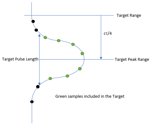
Figure 1. Characteristics of a single target peak envelope.
where:
c is the SoundSpeed (ms-1) read from the echosounder data file.
τ is the PulseDuration (ms) read from the echosounder data file. In range space, the pulse length (m) is cτ/2 and one half of the pulse length is cτ/4.
Target range (m) is the range of the single target.
Target Peak Range (m) is the range of the target envelope's nominal Target Peak TS for single targets derived from TS data. Note: for single targets derived from pulse compressed TS data, the Target range is the Target Peak Range and Tau is the PulseCompressedEffectivePulseDuration (s).
where:
Nominal target peak TS (dB) is the TS (dB) at the Target Peak Range (m).
Target Peak Range (m) = Target Range (m) + cτ/4
Target pulse length defines:
- the start range and stop range of the single target, see TargetPulseLengthm
- the samples that contribute to the single target and samples used for Sv integration, see Integration sampling volume.
Intersection TS (dB) value for TargetPulseLengthm is Nominal target peak TS (dB) - PLDL (dB). Refer to Figure 1 to visualize.
where:
PulseLengthPLDL_Normalized is the unitless value for the normalized PulseLength at the PLDL for the target. PulseLength is normalized against cτ/2. For single target detection variables, PLDL is a Single Target Detection setting on the Variable Properties dialog box. Normalized Pulse length values from detected single targets are displayed under Target on the Details dialog box. The Integrate samples using: list allows you to specify other types of PulseLength for Calibration Assistant calculations.
The PLDL value is theoretically and in-practice a nominal 6dB under Echoview single target detection; the value can be changed but rarely is changed. Other pulse length options include:
Integrate samples using:
Description
Transmitted pulse length
TargetPulseLengthm is cτ/2
Target length at 6dB
Intersection TS(dB) value for TargetPulseLengthm is Nominal target peak TS (dB) - 6dB
TargetPulseLengthm = TargetLengthAt6dBNormalized x cτ/2
Target length at 12dB
Intersection TS(dB) value for TargetPulseLengthm is Nominal target peak TS (dB) - 12dB
TargetPulseLengthm = TargetLengthAt12dBNormalized x cτ/2
Target length at 18dB
Intersection TS(dB) value for TargetPulseLengthm is Nominal target peak TS (dB) - 18dB
TargetPulseLengthm = TargetLengthAt18dBNormalized x cτ/2
Integration sampling volume
The Calibration Assistant uses an integration sampling volume to calculate SaTarget that in turn is used for the calculation of SvOffsetNew and SaCorrectionNew.
The integration sampling volume is centered on the single target peak:
where:
Rt is the target range (m)
c is the SoundSpeed (ms-1) on the Calibration page of the Variable Properties dialog box
τ is the PulseDuration (s)
τe is the equivalent pulse length which is defined as:
τ if Transmitted pulse length is selected under Integrate samples using: or if the EffectivePulseDuration calibration setting is not defined.
The value of EffectivePulseDuration if any of Target length at PLDL, Target length at 6dB, Target length at 12dB or Target length at 18dB is selected under Integrate samples using and the EffectivePulseDuration calibration setting is defined.
τn is the nominal normalized pulse length defined by Target length at PLDL, Target length at 6dB, Target length at 12dB or Target length at 18dB if selected under Integrate samples using, else 1.
Single target detection (Method 1)
The Method 1 Single Target Detection Operators are not recommended for use with the Calibration Assistant, but are supported by Echoview. These operators introduce a special consideration for definition of the integration window. The key change for Method 1 detected single targets derives from the way in which target range is defined.
Single targets have range, Rt, as a property and an integration window must be defined on the basis of that range. The target range is defined on the basis of a nominal echo midpoint, Method 2 and 1 differ as follows:
- Method 2:
- The envelope is defined using a PLDL (Pulse Length Determination Level), nominally 6dB
- The echo midpoint is taken as the power weighted mean of sample ranges in the envelope
- The target range is cτ/4 lower than the echo midpoint (i.e., one half of the transmitted pulse length)
- Method 1:
- The envelope is defined using a PLDL (Pulse Length Determination Level), nominally 6dB
- The target range is taken to be the range of the first sample in the envelope
- This is, by definition, based on the PLDL not the transmitted pulse length
- We can infer the midpoint of the envelope from the target range less half the PLDL envelope width
The generalized definition of the integration window thus becomes:
where:
Rt is the target range (m), a property of single targets in Echoview
c is the sound speed (ms-1) on the Calibration page of the Variable Properties dialog box
τm is the transmitted PulseDuration τ (s) except for Method 1 single targets when it is the PLDL pulse length τPLDL, where:
τPLDL is the Echoview PulseLength_Normalized_PLDL property of single targets. The EffectivePulseDuration is never used in this context even when available.
τe is the equivalent pulse length which is defined as:
τ if Transmitted pulse length is selected under Integrate samples using or if the EffectivePulseDuration calibration setting is not defined
The value of EffectivePulseDuration if any of Target length at PLDL, Target length at 6dB, Target length at 12dB or Target length at 18dB is selected under Integrate samples using and EffectivePulseDuration calibration setting is defined
τn is the nominal normalized pulse length defined by Target length at PLDL, Target length at 6dB, Target length at 12dB or Target length at 18dB if selected under Integrate samples using, else 1.
Off-axis angle
Single targets with angular position data can use a specified Off axis angle as a boundary condition for on-beam-axis targets. A target off-axis angle that is less that the Off-axis angle is categorized as on-axis.
See also Off-axis angle equation.
Drop in TS from maximum value (dB)
The On-Axis Definition relies on the specified Drop in TS from the maximum value (dB) as a boundary condition for on-axis targets. The TS maximum (dB) is defined as the peak uncompensated TS of the set of single targets in the region or selection.
The peak uncompensated TS is:
- likely to be close to the beam axis, where the transducer gain is greatest (and beam compensation is zero). See Beam pattern illustration, Typical beam pattern.
- the best representative of the TS of the calibration sphere
As target uncompensated TS deviates from the peak TS (of the set of targets), the target angular position deviates from the beam-axis (0, 0).
Things to consider when estimating a "Drop in TS" value:
- A drop of 3dB is a halving of power.
- The general behavior of uncompensated TS for Calibration sphere data that includes angular position. Refer to Figure 3 minor-axis beam compensation graph and Figure 4. Off-axis beam compensation graph.
- Transducer specification beam pattern data.
- The RMS Error value calculated by the Calibration Assistant.
TS & Sv Offsets / Gain & Sa Correction
Control the type of TS & Sv Offsets / Gain & Sa Correction using the Calibration Assistant.
TS Offset
where:
TSoffsetNew is the generic constant CalibrationOffsetTS that is required to match the Sphere Data TS to the mean on-axis TS of single targets in the region or selection.
TSoffsetCurrent is the current value for CalibrationOffsetTS read by Echoview.
SphereDataTS is the Sphere Data TS (dB) value.
MeanOnAxisTS is the mean TS (dB) of the on-axis single targets in the region or selection. The mean is calculated in the linear domain and converted back to dB.
Sv Offset
The Sv offset is evaluated using the theoretical calibration sphere Sv and TS values and on-axis Sv data associated with each on-axis single target.
where:
SvOffsetNew is the CalibrationOffsetSv value required to match the theoretical SvCalSphere to the mean of the sample Sv contributions from the on-axis calibration sphere single targets.
SvOffsetCurrent is the Current CalibrationOffsetSv read by Echoview from the echosounder data file or ECS file.
Mean[SvOffsetcurrent + Sasphere - Satarget] is the mean calculated in the linear domain and then re-expressed as a dB value. Each [SvOffsetcurrent + Sasphere - Satarget] value is calculated in the dB domain for each on-axis single target in the region or selection. See Sasphere, Satarget.
TransducerGain
This TransducerGain equation is a dB domain version of the ICES CRR 326 Calibration of acoustic instruments (2015) equation 4.8.
where:
TransducerGainNew is the new value for the Simrad TransducerGain (dB) that is required to match the Sphere Data TS to the mean on-axis Simrad TS of single targets in the region or selection.
TransducerGainCurrent is the Current Transducer gain (dB) value.
Sa Correction
The Sa correction is evaluated using the theoretical calibration sphere Sv and TS values and on-axis Sv data associated with each on-axis single target.
where:
j is the index (1, Count) for an on-axis target. Count is a Calibration Assistant Target Summary value.
i is the index for the Sv samples corresponding to an on-axis target envelope for target (j).
SaSphere
Using the expression for the theoretical Sv of a calibration sphere and the relationship between the Area backscattering coefficient and the Area backscattering strength we can express the Sa of a calibration sphere as:
(1)
where:
SaSphere(j) is a theoretical value in dB re 1 m2m-2. It can be calculated for each on-axis calibration sphere single target (j).
RangeSphere(j) is the single target (j) range value in m.
TSSphere(j) is the Calibration Assistant Sphere Data TS (dB) value.
TwoWayBeamAnglecorrected is the Sound speed Corrected two-way beam angle (dB re 1 sr). See Two Way Beam Angle equation.
SaTarget
The expression for SaTarget(j) considers the samples that correspond to the on-axis single target (j) and is the integral of the Sv values within the target's envelope.
On-axis single target properties define the samples that are included for the on-axis target envelope.
(2)
where:
Svcorrected is the corrected Sv dB re 1 m2m-2 of a sample in the on-axis single target envelope.
Svdata is the contributing sample Sv dB re 1 m2m-2 read from the specified Calibration Assistant Sv variable.
TwoWayBeamAngledata is the entry for Manufacturer Data Two Way Beam Angle (dB re 1 sr).
(3)
where:
SaTarget(j) dB re 1 m2m-2 is the ecibel form of the integrated Sv values within the envelope of on-axis single target (j) (specified by the Integrate samples using: list selection).
svCorrected(i,j) is a linear Svcorrected value for sample (i) from the envelope of on-axis single target (j)
SampleSpacingm is the sample thickness (m) derived from the echosounder data.
SaCorrection
The SaCorrectionNew equation is a dB domain version of the ICES CRR 326 Calibration of acoustic instruments (2015) equation 4.9.
(4)
where:
SaTarget is the array of area backscattering strengths dB re 1 m2m-2 calculated using the Sv samples that correspond to each on-axis single target in the region or selection. It represents the numeric integral of Sv over the integration window as specified by the Integrate samples using: value on the Calibration Assistant. See also equation (3) and Integration sampling volume.
SaSphere is the array of area backscattering strengths dB re 1 m2m-2 of the calibration sphere for each on-axis single target in the region or selection. See equation (1).
SaCorrectioncurrent is the Current Sa correction (dB) value read from the echosounder data file or ECS file.
Mean[...] is the mean calculated in the linear domain and then re-expressed as a dB value.
TransducerGainCurrent is the Current Transducer gain (dB) value read from the echosounder data file or ECS file.
TransducerGainNew is the new value for the Simrad TransducerGain (dB) that is required to match the Sphere Data TS to the mean on-axis Simrad TS of single targets in the region or selection. See Transducer Gain equation.
Angle Offsets and 3dB beam angles
On-axis Sv and TS calibration are concerned with tuning the on-axis calibration sphere measurements. The process ensures the average of the on-axis peak TS measurements are calibrated with respect to the theoretical calibration sphere TS.
Angle offsets and 3dB beam angle calibration are concerned with tuning four* beam compensation angle parameters. The process that calibrates the angle offsets ensures the average of the on-axis peak TS occurs at α = β = 0. The angle offsets are used to center the beam pattern compensation on the beam axis. The process that calibrates the 3dB beam angles scales the width of beam pattern.
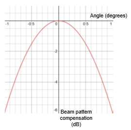
Figure 2. A typical beam pattern. The beam axis is at α = β = 0 degrees.
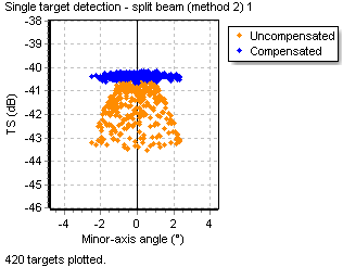
Figure 3. On-axis calibration sphere single targets plotted on a Minor-axis beam compensation graph.
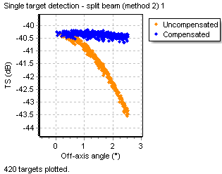
Figure 4. Off-axis angles of calibration sphere single targets plotted on the Off-axis beam compensation graph.
Figure 2 displays a typical beam pattern.
where:
- α is the Minor-axis angle (degrees)
- β is the Major-axis angle (degrees)
- δα is the Minor-axis offset angle (degrees)
- δβ is the Major-axis offset angle (degrees)
- Minor-axis 3dB beam angle (degrees) is the angle at the half power point which is 3dB down from zero beam compensation.
- Major-axis 3dB beam angle (degrees) is the angle at the half power point which is 3dB down from zero beam compensation.
- TS(a, b) = uncompensated TS of the on-axis calibration sphere single target + Beam compensation model correction (a, b).
Within the Calibration Assistant, a variety of beam compensation graphs can be displayed beside Target Summary statistics. The graphs can help in the observation of calibration sphere data trends and problems.
Figure 3 Uncompensated TS data points show a typical beam pattern for the main lobe of a transducer. The compensated TS data points can indicate how well the beam compensation model corrects the uncompensated TS. Theoretically, the mean of the compensated on-axis TS should equal the TS of a 23 mm copper calibration sphere (TS = -40.40 dB). A similar pattern is observed in the Major-axis beam compensation graph (not shown). The minor- and major-axis offset angles help center the single target values around the beam axis.
In contrast, Figure 4 plots the single target off-axis angle against the compensated and uncompensated TS. The advantage of this graph is that curves for TS are clear and simple. The uncompensated TS values sit on a curved line and the compensated TS values describe a straight line whose mean is the TS of the calibration sphere. Departures from well-behaved beam compensation are easier to see with this graph. The graph is suited to data from circular transducers. Elliptical transducer data interpretation is affected by the magnitude of the angle difference between the major and minor-axis angles.
New angle offset and 3dB beam angle values rely on these assumptions:
- the beam compensation is calculated for any target, using the single target's angular position
- the beam compensation added to the single target uncompensated TS value equals a mean TS value which is the same for all on-axis calibration sphere single targets
- the boundaries of validity for the beam compensation model
- *The BioSonics and Simrad LOBE beam compensation models express the beam compensation as a function of single target major and minor-axis angles and transducer major and minor-axis 3dB beam angles. For such models four angle parameters can be estimated when 3dB beam angle data are available. Otherwise, only two angle offsets can be estimated.
Notes:
- For the Simrad Specific Output format the Simrad angle equation subtracts the AngleOffset.
- For the Generic Output format the BioSonics angle equation adds the AngleOffset.
- See also: Target Summary graphs.
Angle offset and 3dB beam angle solution iteration
RMS Error
RMS (Root Mean Square) Error is a measure of how close the single target TS data is to the TS maximum when evaluated under the new Angle offsets and 3dB beam angles. A value close to zero means that the set of compensated TS is close to the peak TS of the set. When the RMS Error is large, review your Calibration Assistant region/selection, Input Values and On-Axis Definition.
where:
n is the number of single targets in the selection/region.
TSi is the TS of the ith single target in the selection/region.
𝔼(TS) is Expected TS of the calibration sphere
The RMS Error is calculated in the dB domain.
Using the properties of a well-formed beam pattern shape and the knowledge that peak TS is at α = β = 0 degrees, iterations for δα, δβ, Minor-axis 3dB beam angle and Major-axis 3dB beam angle are conducted in a stepwise process until the RMS error is minimized (ie., closer to zero).
For each variable (V) [α, β, δα, δβ] Echoview fits a model through an iterative process to evaluate new calibrated values for V [α, β, δα and δβ]. In theory, Echoview's steps in fitting the model include:
- Defining the constants:
- Δ = 0.5
- γ = 10-5
- V0 as the current value of the variable V
- 3dB beam angle iteration, with the angle offsets (δα, δβ) held constant.
- Echoview calculates through nine RMS Error 'axis positions' (e.g., 'α, β', 'α, β + Δ'...).
- Selects the position with the lowest RMS Error, set V0 to the respective position value:
- If it is α, β then halve Δ, and the model loops back to 2a.
- if Δ < γ accept V = V0 as the solution, or,
- Else loops back to 2a.
- Angle offset iteration, with dB beam angles (α, β) held constant.
- Echoview calculates through nine RMS Error 'axis positions' (e.g., 'δα, δβ', 'δα, δβ + Δ'...).
- Selects the position with the lowest RMS Error, set V0 to the respective position value:
- If it is δα, δβ then halve Δ, and the model loops back to 3a.
- if Δ < γ accept V = V0 as the solution, or,
- Else loops back to 3a.
References
Simrad AS 2003a. Instruction manual. Simrad EK60 Scientific echosounder system. 91 p. ISBN 82-8066-012-7.
Simrad AS 2003b. Operator manual. Simrad ER60 Scientific echosounder system. 166p. ISBN 82-8066-011-9.
See also
Calibration Assistant dialog box
Major-axis beam compensation graph
Minor-axis beam compensation graph
Beam geometry
About single targets
Single target detection operators
About calibrated data
Echoview calibration supplement files