Time Series Properties dialog box

Raw Time Series Properties pages

Editable Line Properties pages

Virtual Time Series Properties pages

Display
Calibration
Visibility
Name and Notes

Source
Display
Visibility
Name and Notes

Alongtrack Display
Arithmetic
Best Bottom Candidate Line Pick
Code - Time Series
Crop
Display
Fixed Depth line
Interval Analysis - Bottom Feature
Interval Analysis - Calibration
Interval Analysis - Single Targets
Interval Analysis
Linear Offset
Maximum Sv Line Pick
Near-field Depth
Name and Notes
Off-Axis Angle Offset
Operands
Regions
Solar Elevation At Pings
Span Gaps
Smoothing Filter
Statistical Combination
Threshold Offset
Time Offset
Time Series Select
Time Series Set Status
Towed Body Time Offset
Trained Model Bottom Exclusion (experimental)
Transmission Time Series Select
Type Conversion - Time Series
Visibility

Settings

Description

Operator Type

The operator that is being applied to create the virtual line or virtual time series. This cannot be changed.

Operand(s)

The line, lines or variables/time series that are used to create the virtual time series. Use the Operand list arrow to select an operand.

When available click Add New Operand to add an operand or click Remove Last Operand to remove an operand.

Description

A large text box that displays a summary of the selected operator, including applicable data types, Dataflow Toolbox category/categories, and required Echoview modules.

Settings

Description

Line source

Specifies the line source used when:

• a line is automatically extended as new data arrives during live viewing
• a line is recalculated using Recalculate Line on the echogram Shortcut menu.

The line source list can include:

Offset

Specifies the type of line offset to apply to the Offset line.

Select one of:

General

• Span gaps

Select Span gaps to span gaps in the line.

If the extension is based on a sounder-detected bottom and depth data does not arrive as expected, the extension will stop until depth data is received at which point a line segment with a line status of Unverified will connect the last received depth to the new one.

If the extension is based on another line then any gap in that line will be bridged (in the extension to this line) by a line segment with a line status of Unverified.

Otherwise, this option has no effect.

Setting

Description

Transducer

The sounder-detected bottom line is associated with a transducer. Select a Transducer from the Transducer list. A Transducer object in the Dataflow window allows you to configure a transducer. The Transducer Properties allow you to record general information, and enter settings for transducer location and orientation.

Edit the calibration file used by this fileset

This hyperlink is only available when an ECS file has been added to the fileset. Use the hyperlink to Edit the ECS file.

Note: An ECS file may affect multiple EV files or multiple variables. For more information refer to Echoview Calibration Supplement files.

Refer to the SourceCal entry.

Refer to the LocalCal entry.

Displays calibration settings that Echoview uses for calculations.

Echoview handles an extensive range of calibration settings, a complete list (including default values, units and ranges) can be found under Help menu > Calibration Information. Only a subset of these are relevant to your data. Echoview knows a setting is relevant when it reads it from a data or ECS file, or uses it in a calculation. These are the ones that were read from the variable's own calibration source in the data file, or explicitly associated with the fileset or calibration source in the ECS file.

The Time Series Properties Calibration page only displays the calibration settings that are relevant to the raw line variable.

The Used by segments section displays the applicable line segments for the displayed calibration settings.

The Value column lists the values used in calculation.

The Calibration file column lists the values read from the ECS file in the fileset.

The Data file column lists the values read from the data files in the fileset.

For a technical description of the various calibration settings please consult:

• Common calibration setting names
• Transducer specific calibration setting names

Notes:

• The setting colors are based on the processing that has been done since the data and ECS files were last loaded. If you reload the ECS file, after changing some values for example, you may find that some settings revert to grey. This is because Echoview has not found the need to use them since the reload. Recalculate or step through the pings in the echogram to use any newly modified settings.
• You can copy displayed Calibration settings and paste them into an ECS file.
• A warning message is sent to the Messages dialog box when the calibration settings read from the data files in the fileset vary between pings. There will then be more than one Used by segments group. With respect to the line variable, it is the line points and as a result line segments that are affected by ping calibration.

Settings

Description

Show transects

Visualize transects on the cruisetrack display.

Show transect labels

Display the transect name.

Show grid

Check this box to display grid lines on the alongtrack display, and leave it unchecked to view the display without grid lines.

Note: This setting will only affect the alongtrack display, and not any open echogram.

Show scale bar

Select to display the scale bar.

Show zoom controls

Select to display zoom controls.

Show synchronized position

Select to display the cross-hair position when auto-synchronized.

Show color legend

Select to display the alongtrack color legend.

Settings

Description

Line

Select Line to display time series values on an alongtrack line in a cruisetrack window.

Bubbles

Select Bubbles to display time series values as proportionate circles on the cruisetrack in a cruisetrack window.

The bubble diameter in pixels is specified using a minimum and maximum diameter to map to the range of time series values.

• Minimum bubble diameter (pixels)
• Maximum bubble diameter (pixels)

Track thickness

By default the alongtrack thickness is specified by the Track thickness on the Cruisetrack page of the EV File Properties dialog box.

Select Use custom thickness and specify a thickness value to override the setting on the EV File Properties dialog box

Settings

Description

Color display minimum

Sets the value below which all data values will be displayed in the Below threshold color of the selected color scheme.

Color display range

Sets the range of data values which are mapped to the selected color scheme. All values above (Color display minimum + Color display range) will be displayed in the color scheme's Above (threshold + range) color.

Color scheme

Use the Color scheme list to choose from predefined or customized color schemes.

Select Use alternate color scheme to display the alternate version of the selected Color scheme.

User-defined color schemes can be created and edited with the Echocolor application supplied with Echoview. Note that if you add, remove or change the color scheme files in this folder you will need to restart Echoview before those changes take effect.

The grid color is determined by the alongtrack color scheme, unless overridden by Custom > Grid color on the Cruisetrack Display page of the EV File Properties dialog box.

Note: If a user-created custom color scheme has the same name as a predefined color scheme, its name will have " (.evc file)" appended to it to denote this. See About color schemes for further information.

Settings

Description

Default

Select Default to use the default time series segment thickness and status color specified under the Time Series page of the EV File Properties dialog box.

Custom

Select Custom to specify the custom time series segment thickness and color.

Thickness

Specifies the displayed segment thickness in pixels for the time series variable.

Time series colors

Specifies the time series status colors of displayed segments for the time series variable.

Click a status color to display a color palette and choose a new color.

Unit name

This section is displayed for time series select variables with a time series data type selected as Unspecified data type.

Enter the text for a Unit name. This name may be used on Graphs and Tables. When a Unit short name exists, the short name is used instead.

Unit short name

This section is displayed for time series select variables with a time series data type selected as Unspecified data type.

Enter the text for a Unit short name. When a Unit short name is available, it is used on Graphs and Tables.

Setting

Description

Dynamic name

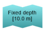
Select Dynamic to use a name that updates when a Line Property updates. Some lines have a default Dynamic name - indicated by text with a property name inside braces (curly brackets). The Properties Information window displays supported Command interface property names. Suitable property names are those that have numeric or text value. A Dynamic name may be specified through the Console with the Properties option DynamicName.

When Dynamic is selected, the Name property becomes read-only under the Command interface and the dataflow object.

Example: A Fixed depth line has a default Dynamic name of Fixed depth [{Depth} m] that is displayed on the line object in Figure 1 - the Depth value is 10.0 m. When the value for Depth changes, the Dynamic name updates automatically.

Figure 1.

Notes:

• Refer to Fileset rename note.
• Refer to Console Property option DynamicName.
• A dynamic name may become invalid when property names are incorrect, deprecated, or no longer recognised by Echoview. In many cases Echoview displays a warning and converts the invalid {property name} to plain text by removing the braces. If necessary, use Reset to regenerate the default dynamic naming using the current property names. See also Known issues: Dynamic name warning.
• When using the Multiple Object Properties dialog box, Dynamic is disabled. To assign a new name, edit objects individually.

Reset

Use Reset to reassign a default Name or regenerate the default Dynamic name using the current property names.

Name

Default assigned name or enter text to specify a name. See also: Notes for name uniqueness and supported characters in a name.

Note: When using the Multiple Object Properties dialog box, Name is disabled. To assign a new name, edit objects individually.

Data type

Displays the data type of the output virtual variable.

Notes

Section for notes including line pick settings.

Setting

Description

Start depth (m)

Determines at what depth (m) the Line picking algorithm will start, i.e., data above this depth will not be considered.

This is particularly useful if you have high return areas at the top of your echogram that you wish to avoid being picked as bottom.

Stop depth (m)

Determines at what depth (m) the Line Picking algorithm will stop i.e., data below this depth will not be considered.

Minimum Sv for a good pick (dB)

See Best bottom candidate settings description for details.

Use Backstep

When checked the Discrimination level and Backstep range settings are available.

Discrimination level (dB)

See Best bottom candidate settings description for details.

Backstep range (m)

See Best bottom candidate settings description for details.

Peak threshold (dB)

See Best bottom candidate settings description for details.

Maximum dropouts (samples)

See Best bottom candidate settings description for details.

Window radius (samples)

See Best bottom candidate settings description for details.

Minimum peak asymmetry

See Best bottom candidate settings description for details.

Setting

Description

Python source file

Specifies the path and file name of an Echoview Python source file.

Use ... to browse to and open a Python file.

Use New to create a new Python file.

Use Edit to edit the Python source file.

Click X to remove a Python file.

Notes:

• Use (Python) Editor on the General page of the Echoview Configuration dialog box to specify an editing application other than Windows Notepad.
• To use additional Python packages with Echoview, set the required Windows environment variable at the Command Prompt before opening Echoview. See Using other packages with Echoview.

Window size (pings)

Specifies the number of pings the Code - Time series operator processes per iteration.

Valid inputs are odd integers greater than or equal to 1.

See Using the window of measurements for details.

Arguments

Lists the named argument values that Echoview passes to the Operator class’s __init__ method in the selected Python source file.

Each argument added here must have a corresponding parameter in __init__. Echoview does not automatically add the parameter to the Python source file. If a corresponding parameter is not declared, the script cannot run.

Use Add... to enter an argument name and value in the Code Argument dialog box.

• Name – Enter a valid Python parameter name containing letters, numbers, or underscores. The name must not begin with a number, contain spaces, or be a Python reserved word, and must be fewer than 255 characters.
• Value – Enter a numeric value without spaces or a string enclosed in double quotation marks. The Python source file is responsible for interpreting and, where necessary, converting the value.

Examples:

• -6 is passed as a numeric value and displayed as -6.0.
• 37.9 is passed as a numeric value.
• "6 degrees of freedom" is passed as a string.
• - 6 is passed as a string because it contains a space and may therefore produce an unexpected result.
• A blank value is passed as an empty string, even when the corresponding __init__ parameter has a default value.

Use Edit..., or double-click an argument, to edit it in the Code Argument dialog box.

Use Delete to delete the selected argument.

For more information, see Arguments.

Settings

Description

Minimum value

Specifies the minimum value to crop the operand.

Maximum value

Specifies the maximum value to crop the operand.

Setting

Description

Start depth

Determines at what depth (m) the Line picking algorithm will start, i.e., data above this depth will not be considered.

This is particularly useful if you have high return areas at the top of your echogram that you wish to avoid being picked as bottom.

Stop depth

Determines at what depth (m) the Line Picking algorithm will stop, i.e., data below this depth will not be considered.

Minimum Sv for good pick (dB)

This setting specifies the minimum Sv (dB) value for good line status for the Line pick algorithm.

Use Backstep

When checked the Discrimination level and Backstep range settings are available.

Discrimination level

Specifies the Discrimination level (dB) for the Maximum Sv algorithm.

Backstep range

Specifies the Backstep range (m) for the Maximum Sv algorithm.

Setting

Description

Depth

Enter the depth, in meters, of the virtual line.

Settings

Description

Use time/distance grid interval from operand 1

Select this grid to use for the bottom feature calculation. Otherwise the virutal variable inherits the grid settings from the input acoustic variable.

Custom grid interval

Select this grid to use for the bottom feature calculation. This grid allows you to specify a grid independently of the operand.

Show time/distance grid

Select the analysis interval to use. Options include:

• Ping number
• Time (minutes, hours, or days)
• GPS distance (nmi or m)
• Vessel log distance (nmi or m)
• Water current distance (m)

Spacing between grid lines

The name of this setting updates in response to the selected interval type. Enter a value appropriate to the unit shown.

Interval names include:

• Ping number: Number of pings between grid lines
• Time (minutes): Time between grid lines (minutes)
• Time (hours): Time between grid lines (hours)
• Time (days): Time between grid lines (days)
• GPS/Vessel log distance (nmi): Distance between grid lines (nmi)
• GPS/Vessel log distance (m): Distance between grid lines (m)
• Water current distance (m): Distance between grid lines (m)

Feature

Specifies a single bottom feature to extract:

• Bottom hardness normalized
• Bottom kurtosis
• Bottom line depth mean
• Bottom maximum Sv
• Bottom rise time normalized
• Bottom roughness normalized
• Bottom skewness
• First bottom length normalized
• Second bottom length normalized

Notes:

• Known issue: a feature may return no value for an interval, and a value of 0 is assigned. This may cause an issue when 0 could be a valid value for the feature.
• Bottom maximum Sv, Bottom kurtosis, Bottom skewness are associated with the first bottom echo. These features may reveal useful characteristics of the roughness index that is used to calculate Bottom roughness normalized.
• When no second bottom echo exists, the calculation for Second bottom length normalized and Bottom hardness normalized can't be evaluated.
• See also: About bottom classification, Bottom classification algorithms.

Setting

Description

Calibration setting

Select a setting from the Calibration setting list. Supported calibration settings may be included in the settings displayed for a new but empty EV file, under Help menu, Calibration Information list.

Note: Known issue: a calibration setting may return no value for an interval, and a value of 0 is assigned. This may cause an issue when 0 could be a valid value for the setting.

Setting

Description

Use time/distance grid interval from operand 1

Select this grid to use for the single target calculation. Otherwise, the virtual variable inherits the grid settings from the input acoustic variable.

Custom grid interval

Select this grid to use for the single target calculation. This grid allows you to specify a grid independently of the operand.

Show time/distance grid

Select the analysis interval to use. Options include:

• Ping number
• Time (minutes, hours, or days)
• GPS distance (nmi or m)
• Vessel log distance (nmi or m)
• Water current distance (m)

Spacing between grid lines

The name of this setting updates in response to the selected interval type. Enter a value appropriate to the unit shown.

Interval names include:

• Ping number: Number of pings between grid lines
• Time (minutes): Time between grid lines (minutes)
• Time (hours): Time between grid lines (hours)
• Time (days): Time between grid lines (days)
• GPS/Vessel log distance (nmi): Distance between grid lines (nmi)
• GPS/Vessel log distance (m): Distance between grid lines (m)
• Water current distance (m): Distance between grid lines (m)

Analysis variable

Specifies a single target analysis variable to extract:

• Beam volume sum
• Target count
• Target depth mean
• Target length mean
• Target range mean
• Thickness mean
• TS maximum
• TS mean
• TS minimum
• Wedge volume sampled

Note: Known issue: an analysis variable may return no value for an interval, and a value of 0 is assigned. This may cause an issue when 0 could be a valid value for the analysis variable.

Setting

Description

Use time/distance grid interval from operand 1

Select this option to use the time/distance grid interval from operand 1 to calculate the selected analysis variable.

Custom grid interval

Select this option to specify a time/distance grid interval independently of the operand.

Show time/distance grid

Select the analysis interval to use. Options include:

• Ping number
• Time (minutes, hours, or days)
• GPS distance (nmi or m)
• Vessel log distance (nmi or m)
• Water current distance (m)

Spacing between grid lines

The name of this setting updates in response to the selected interval type. Enter a value appropriate to the unit shown.

Interval names include:

• Ping number: Number of pings between grid lines
• Time (minutes): Time between grid lines (minutes)
• Time (hours): Time between grid lines (hours)
• Time (days): Time between grid lines (days)
• GPS/Vessel log distance (nmi): Distance between grid lines (nmi)
• GPS/Vessel log distance (m): Distance between grid lines (m)
• Water current distance (m): Distance between grid lines (m)

Analysis variable

Specifies a single analysis variable to calculate for the specified interval.

The Analysis variable list displays all options. If the selected analysis variable does not support the data type of the operand, Echoview displays a warning in the Messages dialog box when the calculation is required. This may occur when displaying a graph, table, or alongtrack feature, or when exporting the time series. The calculation may produce either no output or no data values.

For onscreen calculations, the analysis variable does not need to be selected under the Integration results folder on the Export page of the EV File Properties dialog box.

For exports using the Sample analysis exporter, select the required analysis variables in the applicable export settings. Refer to Exporting integrations for information about calculation output and associated analysis statistics.

Operands of data type Sv are supported by the following analysis variables:

• ABC
• Aggregation index
• Area backscatter strength
• Beam volume sum
• Center of mass
• Equivalent area
• Inertia
• Mean exclude above depth
• Mean exclude below depth
• NASC
• Proportion occupied
• Sample kurtosis
• Sample skewness
• Sample standard deviation
• Sv maximum
• Sv mean
• Sv minimum
• Thickness mean

Known issue note: An analysis variable may return no value for an interval, in which case a value of 0 is assigned. This may cause an issue when 0 is a valid value for the analysis variable.

Operands of data type dB are supported by the following analysis variables:

• Mean exclude above depth
• Mean exclude below depth
• Sample kurtosis
• Sample maximum dB
• Sample mean dB
• Sample minimum dB
• Sample skewness
• Sample standard deviation

dB operand note: For some analysis variables, dB data is converted to its linear equivalent for the calculation and then converted back to dB for the output.

Operands of data type Linear are supported by the following analysis variables:

• Mean exclude above depth
• Mean exclude below depth
• Sample kurtosis
• Sample maximum
• Sample mean
• Sample minimum
• Sample skewness
• Sample standard deviation

Standard deviation, Skewness and Kurtosis note: Standard deviation, Skewness and Kurtosis contain expressions in the denominator that can cause the calculation to be undefined. Echoview sends a message when this becomes the case.

Settings

Description

Multiply value by

Enter a value to multiply the time series by.

Then add

Enter a value to add to the resulting time series value.

Settings

Description

Multiply near-field range by

This is a factor by which to extend the near-field range that Echoview computes. The multiplier is applied in the range dimension then values are converted to depth. The default value is 2.

Settings

Description

Transducer

Select the transducer that will be used in the off-axis angle offset calculation.

Angle (degrees)

Enter the angle, in degrees, that will be used to apply an off-axis offset to the input operand.

Settings

Description

Line status

Sets the selected line status for the bridging line segments in the virtual line.

Maximum gap size (seconds)

Sets the maximum time between gaps to be bridged.

Settings

Description

Smoothing mode

Determines the smoothing applied to the window (whose size is specified by the Number of points) for the operand line.

Select a Smoothing mode:

Number of points (window size)

Specifies the size of the smoothing window for operand time series. Enter an odd number between 1 and 251. A larger smoothing window may increase the processing time.

The applied Smoothing mode determines the output value for each point in the smoothed virtual time series.

Note: A window size of 1 will create a virtual line the same as the operand line; no smoothing will occur.

Settings

Description

Time zone (hours from UTC)

The time zone offset, in hours, used to convert the operand's local time to UTC.

Settings

Description

Statistic

Determines the statistical operation to apply to the operand time series (selected on the Operands page).

Select one of:

Divergence

Check Apply divergence limit to apply a divergence limit to the input values.

Enter a value for Divergence limit.

Divergence is defined as the difference of any one operand's value from the mean of all of the operand values, at a time (T). If any operands have values that exceed the Divergence limit, those time series will be ignored in the calculation of the output time series at time (T).

Settings

Description

Detect minimum threshold

Detect a threshold that is the minimum value (dB) for a boundary. Enter the value under Threshold (dB).

This setting is normally used when the base line to boundary feature varies from high to low dB value.

Detect maximum threshold

Detect a threshold that is the maximum value (dB) for a boundary. Enter the value under Threshold (dB).

This setting is normally used when the base line to boundary feature varies from low to high dB value.

Allow detection from echogram extents

Select this setting when the operand line is beyond the operand variable extents. The Threshold offset algorithm will begin the detection at the operand variable extent.

Apply line-relative smoothing to the echogram data

Select Apply line-relative smoothing to the echogram data to apply a 3x5 Blur convolution with the center of the kernel set to 1. Note that range changes between pings may result in unexpected smoothing.

Smoothing increases the processing time.

Minimum accepted distance (m)

The Minimum accepted distance value specifies a minimum boundary distance for boundary samples. The default value is 0 meters.

A ring down boundary detection benefits from the default value.

A vegetation boundary detection from a bottom line may be more successful with a small non-zero Minimum accepted distance. In this case, areas with a height less than Minimum accepted distance are ignored.

Maximum detection distance (m)

The Threshold offset detection will not detect beyond this specified distance in depth from Operand 2 in the Direction of detection.

Direction of detection

The Direction of detection from the line operand may be specified as Above operand line or Below operand line.

Settings

Description

Time offset

Select the time offset operation. The operator can Add or Subtract the specified time from the operand.

Days

Specify the number of days to offset.

Hours

Specify the number of hours [0, 23] to offset.

Minutes

Specify the number of minutes [0, 59] to offset.

Seconds

Specify the number of seconds [0, 59] to offset.

Milliseconds

Specify the number of milliseconds [0, 999] to offset.

Settings

Description

Select series

Series to select

Use the Series to select list to specify the time series to derive from the Operand 1 time series collection for the virtual variable.

Time series data type

Standard data type

Select Standard data type to assign a data type and its associated interpolation method. Then use the Standard data type list to specify the data type.

Available data types include:

• Depth line (m)
• Depth line values have units of meters. The value -10000.99 is the no data depth value.
• Distance (nmi)
• Distance values (a.k.a. vessel logs) have units of nautical miles. The value -9.9e+37 is a no data distance value.
• Heading (°)
• Heading values have a range of 0 to 360, and units of degrees. The value -9.9e+37 is a no data heading value.
• Length (m)
• Length values have units of meters. The value -9.9e+37 is a no data length value.
• Pitch (°)
• Pitch values have a range of -180 to 180, and units of degrees. The value -9.9e+37 is a no data pitch value.
• Roll (°)
• Roll values have a range of -180 to 180, and units of degrees. The value -9.9e+37 is a no data roll value.
• Speed (m/s)
• Speed values have units of meters per second. The value -9.9e+37 is a no data speed value.
• Solar elevation (°)
• Solar elevation values have a range of -90 to 90, and a unit of degrees. The value -9.9e+37 is a no data solar elevation value.

Unspecified data type

Select Unspecified data type to assign a general-purpose time series data type whose interpretation is user-defined. Use the Interpolation mode list to specify the interpolation method for the values of the custom time series.

Available Interpolation modes include:

• Circular [-180, 180]
• Suited to data with circular -180 to 180 range handling. Has a ‘no data’ value -9.9e+37.
• This interpolation mode is useful for time series similar to pitch and roll.
• Circular [0, 360]
• Suited to data with circular 0 to 360 range handling. Has a ‘no data’ value -9.9e+37.
• This interpolation mode is useful for time series similar to heading.
• Linear
• Suited to data that interpolates linearly between points. Has a ‘no data’ value -9.9e+37.
• This interpolation mode is useful with continuous values, such as depth, temperature, height, etc…
• Stepped
• Suited to data that interpolates in a stepped manner. Has a ‘no data’ value -9.9e+37.
• This interpolation mode is useful for series with discrete values, such as fish counts.
• dB
• Suited to data measured in decibels (dB). Data is converted to linear values, linearly interpolated, then converted back to the dB domain. Has a ‘no data’ value -9.9e+37.

Settings

Description

Status

Specifies the status to assign to the time series measurements selected by the range settings below.

Minimum in-range data value

Enter a desired minimum in-range time series value.

Maximum in-range data value

Enter a desired maximum in-range time series value.

Set status of in-range measurements

Select to change the status of time series values that fall within the specified range (Minimum value to Maximum value).

Set status of measurements outside the range

Select to change the status of time series values that fall outside of the specified range.

Settings

Description

Tow point

X-alongship offset (m)

The platform tow point offset is located from the platform system reference and to the tow point. X axis tow point offset value is in meters. Negative offset values are towards the aft of the platform. For further information refer to the Towed body time offset diagram and assumptions.

Z-vertical offset (m)

Z axis tow point offset value in meters. Negative is up and positive is down.

Tow line

Fixed length (m)

The tow line is relative to the tow point and is in the alongship direction.

Select and specify a value for a fixed tow line length (m).

Varying length (m)

Use the Varying length list to specify a length variable derived from tow line length data.

Settings

Description

Detection start range (m)

The operator does not consider ping samples from above this range (refer to its Line picking algorithm). This allows you to omit phenomena such as the transducer ring down, the near-field zone or surface features as false bottom detections.

Settings

Description

Statistic

Select a Statistic from the list:

• Impedance Median
• Calculates the median of the selected Component data.
• Impedance Interquartile Range
• Calculates the interquartile range of the selected Component data.
• Impedance Maximum
• Determines the maximum impedance for the selected Component data.

Component

Select the Component for the Statistic calculation:

• Transducer
• Statistics for the whole transducer are an aggregate of values from all pings within all sectors.
• Sector number
• Statistics for the transducer sector are an aggregate of values from all pings within the specified sector.

Settings

Description

Standard data type

Select Standard data type to assign a data type and its associated interpolation method. Then use the Standard data type list to specify the data type. Each standard data type has an inherent interpolation mode.

Available data types include:

• Depth line (m)
• Depth line values have units of meters. The value -10000.99 is the no data depth value.
• Distance (nmi)
• Distance values (a.k.a. vessel logs) have units of nautical miles. The value -9.9e+37 is a no data distance value.
• Heading (°)
• Heading values have a range of 0 to 360, and units of degrees. The value -9.9e+37 is a no data heading value.
• Length (m)
• Length values have units of meters. The value -9.9e+37 is a no data length value.
• Pitch (°)
• Pitch values have a range of -180 to 180, and units of degrees. The value -9.9e+37 is a no data pitch value.
• Roll (°)
• Roll values have a range of -180 to 180, and units of degrees. The value -9.9e+37 is a no data roll value.
• Solar elevation (°)
• Solar elevation values have a range of -90 to 90, and a units of degrees. The value -9.9e+37 is a no data solar elevation value.
• Speed (m/s)
• Speed values have units of meters per second. The value -9.9e+37 is a no data speed value.

Unspecified data type

Select Unspecified data type to assign a general-purpose time series data type whose interpretation is user-defined. Use the Interpolation mode list to specify the interpolation method for the values of the custom time series.

Available interpolation modes include:

• Circular [-180, 180]
• Suited to data with circular -180 to 180 range handling. Has a ‘no data’ value -9.9e+37.
• This interpolation mode is useful for time series similar to pitch and roll.
• Circular [0, 360]
• Suited to data with circular 0 to 360 range handling. Has a ‘no data’ value -9.9e+37.
• This interpolation mode is useful for time series similar to heading.
• Linear
• Suited to data that interpolates linearly between points. Has ‘no data’ value -9.9e+37.
• This interpolation mode is useful with continuous values, such as depth, temperature, height, etc…
• Stepped
• Suited to data that interpolates in a stepped manner. Has a ‘no data’ value -9.9e+37.
• This interpolation mode is useful for series with discrete values, such as fish counts.
• dB
• Suited to data measured in decibels (dB). Data is converted to linear values, linearly interpolated, then converted back to the dB domain. Has ‘no data’ value -9.9e+37.